Section 8: Every Label Is a Multiplier - Deep Dive: Metrics, Cardinality & Alerting Within a Minute

Executive Summary: The metrics path takes 10M samples/s into a time-series database built around a stable series identity, an inverted label index, Gorilla-compressed samples at about 1.4 B each, and a 2 h head block in RAM. Rollups keep sums and counts, and latency lives in histograms because percentiles cannot be rolled up. Cost scales with series count, so cardinality needs hard limits. Dedicated evaluators read the freshest data and fit a 51 s worst-case budget from sample to paging provider.

You: "The log path is expensive but degrades gracefully. The metrics path can gain half the fleet's series from one deploy. I'll walk storage, then that failure, then the alert path Dana's page rides on."

Wall One: Inside the TSDB

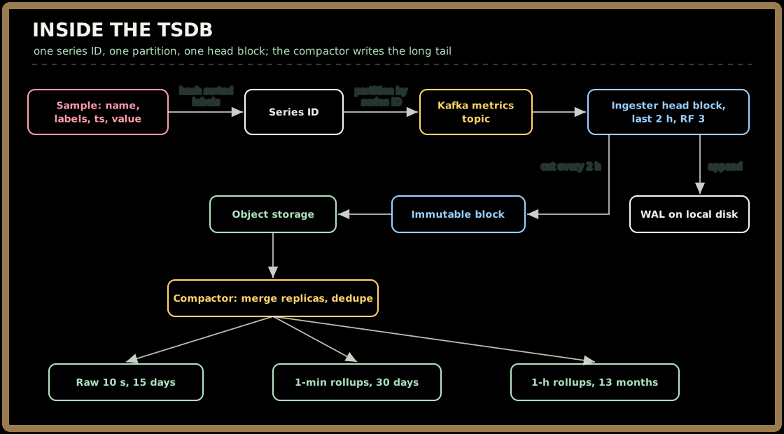
A series is a metric name plus its sorted labels, and its ID is a hash of that string. The gateway computes the ID and Kafka partitions by it (Section 6), so every sample of a series lands on the same ingester partition, replicated RF 3.

Finding series. Each ingester keeps an inverted index: every label=value pair maps to a sorted postings list of series IDs. A selector such as {__name__="http_request_duration_seconds_bucket", service="checkout-api"} fetches two postings lists and intersects them with a linear merge walk. A regex matcher unions the lists of every matching value; a negative matcher subtracts.

Storing samples. A raw sample is a 64-bit timestamp plus a 64-bit float, 16 bytes. Timestamps are stored as delta-of-delta: with a steady 10 s interval the second difference is almost always zero, which costs one bit. Values are XORed with the previous value: an unchanged gauge costs one bit, and a changed one stores only its meaningful middle bits. The result is about 1.4 B/sample, so 864 billion samples a day become about 1.2 TB/day.

The head block. The last 2 h live in ingester memory at about 3 KB per series (samples, labels, index), so 100M series × 3 KB × RF 3 is about 900 GB of RAM across the fleet. Every 2 h the head is cut into an immutable block and flushed; the compactor merges the three replica copies into one, builds larger blocks, and writes rollups. Raw for 15 days (18 TB), 1-min rollups for 30 days (26 TB), 1-h rollups for 13 months (5.7 TB): about 50 TB total.

Why RF 3 if Kafka is durable? Availability, not durability. The WAL plus Kafka can rebuild a 2 h head, but that takes minutes, and every rule on that shard would see a gap. Live replicas keep the alert path inside 51 s through an ingester restart.

Interviewer: "Store a p99 per minute in the rollup. Hourly p99 is then the average of sixty of them."

You: "That number is wrong, not approximate. A p99 is a rank inside a distribution, and keeping only the p99 throws the distribution away. Averaging sixty minute-p99s hides the one bad minute, and averaging p99s across 400 pods is meaningless. So rollups keep min, max, sum and count, which combine exactly (average = sum ÷ count at any level). Latency is stored as a histogram: one counter per bucket boundary. Bucket counts add across pods and across time, and the percentile is computed at query time."

Dana's rule:

histogram_quantile(0.99,
  sum by (le) (rate(http_request_duration_seconds_bucket{service="checkout-api"}[5m]))
) > 0.8      # for: 5m

The price: each bucket is its own series, so a histogram multiplies series count by its bucket count.

Key Insight: Store things that add (counts, sums, bucket counters) and derive things that don't (averages, percentiles) at read time.

Quick check before moving on: