Section 3: The QPS Is Not the Problem - Scale Estimation & Workload Analysis

Executive Summary: This section derives the proximity service's scale in one pass: traffic, writes, corpus, index and shards, caches, logs, bandwidth, and finally regions, failover headroom and node counts. The headline numbers are a 17,400/s search peak, a 400 GB index copy split into 64 shards of 6.25 GB, and 24 search nodes per region. The finding that matters more: raw QPS is modest. The hard part is the work inside each query, because Sam's 1 km covering in Midtown holds 23,600 places.

The interviewer caps the marker. "Before any boxes: how big is this thing?" Assume 100M daily actives worldwide (300M monthly). Now the assumptions become numbers the design must obey, each input said aloud so it can be corrected.

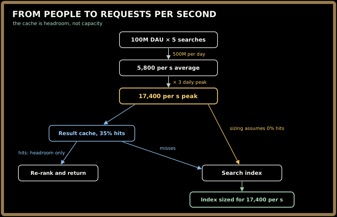
From People to Requests per Second

One rule first: daily peak is 3× the average. Lunch and dinner peak hard in each region, but the world has time zones, so the global curve is smoother than any single city's.

Searches:   100M DAU × 5 searches/day   = 500M/day
            500M ÷ 86,400 s             = 5,787/s ≈ 5,800/s avg
            × 3 peak                    ≈ 17,400/s peak

Details:    0.6 opens per search        = 300M/day
                                        ≈ 3,500/s avg → ~10,400/s peak

Total reads at peak                     ≈ 27,800/s

Geocoding:  20% of searches are "near <text>"
                                        = 100M/day
                                        ≈ 1,160/s avg → ~3,500/s peak
            geocode cache hit rate      = 80%

Five searches sounds high until you count map pans: each drag is a new query.

Interviewer: "The result cache will absorb some of that. Are you sizing the index for the full 17,400?"

You: "Yes. I expect about 35% hits from dense cells, empty and category queries, but that's headroom, not capacity. If the cache goes cold during a failover, the index takes the full load anyway."

Quick check before moving on: