Section 5: One Fact, Two Truths - Data Modeling
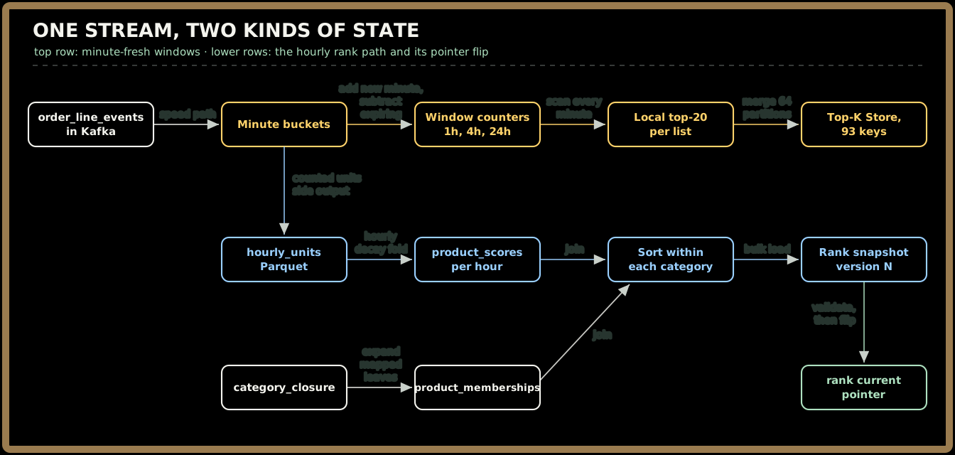
Executive Summary: This section models the data behind ClipKart's Top-10 button and its rank badges, starting from access patterns rather than entities. Everything derives from one immutable fact, the order-line event. The speed path turns it into minute buckets, sliding-window counters and top-20 candidate lists, about 5.6 GB of state that lives inside the stream processor. The rank path turns it into hourly Parquet, a 1.1 GB decayed score table, 200M category memberships and a versioned 8 GB rank snapshot behind a single pointer. Each store gets the alternative it beat and the condition that would flip the choice.
The interviewer turns to a clean section of the whiteboard: "You've got three read APIs. What's actually stored behind them?"
The weak move here is to start drawing entities: Product, Order, Category, Rank. The tables come out tidy and miss the point, because this system has no entities of its own. Orders belong to the Order Service and products belong to the catalog. Everything ranking owns is derived, so the useful question is which derivations it has to answer, and how fast.
Start From the Questions, Not the Nouns
You: "Before I draw any tables, let me list what the system must answer. There are nine questions, and each one picks its own store."
| # | Access pattern | Asked by | Rate / size | Lives in |
|---|---|---|---|---|
| a | Append an order-line event | CDC from checkout | 700/s avg, 15,000/s design peak | Kafka order-line-events |
| b | Units per product per minute | Window Aggregator | ≈ 30,000 products/min | Flink keyed state |
| c | Units per product in last 1h / 4h / 24h | Window Aggregator | 20M live products | Flink keyed state |
| d | Top-20 candidates per (scope, window) | Top-10 API | 93 lists, ~3 req/s behind the shield | Top-K Store (Redis) |
| e | Product → department | Window Aggregator | 200M products | Compacted topic, co-partitioned |
| f | Product → every category it belongs to | Hourly Rank Job | 200M rows | Lake (catalog snapshot) |
| g | Decayed score per product | Hourly Rank Job | 40M rows, 1.1 GB | Lake (Parquet) |
| h | Rank by productId | PDP aggregator, batchGet | ≈ 23k/s at sale peak after cache | Rank Store (Redis cluster) |
| i | Top-100 by categoryId | Best-seller pages | 580/s, 20,000 categories + overall | Rank Store (Redis cluster) |
Read the "Lives in" column top to bottom and it splits into two families. Rows (b) through (e) are minute-fresh, small and owned by the stream. Rows (f) through (i) are hour-fresh, large and owned by the batch job. That's the two-pipeline decision showing up again at the data level. The streaming state is the source of truth for windows, and the lake plus the hourly job is the source of truth for ranks. No metric gets implemented twice: dedup and the per-buyer cap run once, in the Window Aggregator, and the rank path inherits them through the counted units it reads.
Quick check before moving on:
Sign in to continue reading
The rest of this lesson is available with a free account. Signing in with Google or Microsoft is free.
Sign in to read the full lesson