Multi-Source BFS

What is this?

Regular BFS drops one stone in the pond. Multi-source BFS drops a whole handful at once, and lets all their ripples spread together. This is exactly what you want when you ask "how far is each spot from the nearest of several things?" — the closest gym, the nearest fire exit, the time for rot to reach every orange in a crate. Instead of measuring from each source separately and comparing, you let every source flood outward simultaneously, and wherever the ripples meet is the natural dividing line.

💡 Fun fact: image editors use this idea under the name "distance transform" — labeling every pixel with how far it is from the nearest edge or shape. It powers effects like glows and outlines, and it's also how some fonts stay razor-sharp at any size in video games, using "signed distance fields" computed by exactly this many-sources-at-once flood.

🔓 The 2 problems in this chapter are free. Sign in with Google or Microsoft to start solving.

The one-line idea: when you need the distance to the nearest of many sources — or want something to spread from many origins at once — you don't run a separate BFS per source and take minimums. You seed one BFS queue with every source at distance 0 and let a single shared frontier flood outward. One sweep, O(cells), every cell touched once, each labelled by its closest source.

1. What multi-source BFS really means

Standard BFS starts at one node and expands in concentric rings, ring number = distance from that node. Multi-source BFS starts at many nodes simultaneously: all of them are at distance 0, and their rings grow together until the wavefronts meet.

Single-source BFS              Multi-source BFS
(one origin S)                 (origins A and B)

    2 2 2                          A 1 2 2 1 B
    2 1 2                          1 1 2 1 1
    2 1 S 1 2                      2 1 1 1 2
    2 1 2                          2 1 1 1 2
    2 2 2                          1 1 2 1 1
                                   A 1 2 2 1 B

In the multi-source picture, every cell ends up labelled with its distance to whichever source is closest — the two floods meet at a frontier roughly halfway between A and B, and neither side ever overwrites the other, because BFS fills cells in nondecreasing distance order.

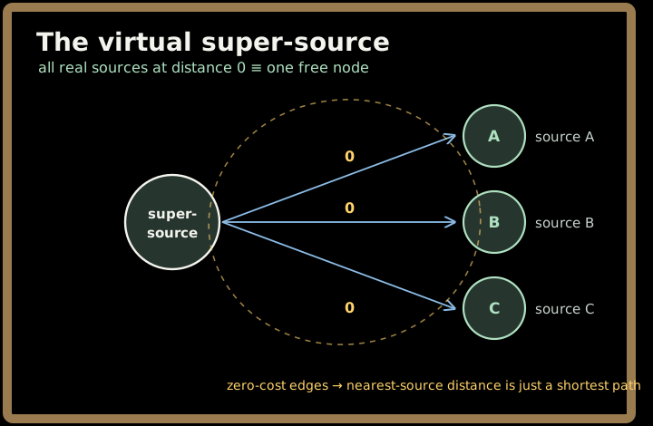
The mental model that makes it click: imagine a single virtual super-source joined by a free (zero-cost) edge to every real source. The shortest path from the super-source to a cell equals the distance to that cell's nearest real source. Seeding the queue with all sources at distance 0 simulates exactly that super-source — which is why one ordinary BFS computes every "nearest-source" distance at once.

Contrast with running BFS from each source separately and taking the minimum: same answer, but O(sources · cells) work and lots of cells written multiple times. The multi-source seed collapses all of that into a single O(cells) frontier.

2. Where you'll actually meet this

"Nearest of many" and "spread from many" are everywhere once you see the shape:

• Distributed systems. Label every node with hops to its nearest cache or replica (read routing, replica placement); model failure or gossip propagation spreading from several origins; assign each region to its closest data centre.
• Logistics. Tag each delivery zone with its distance to the nearest warehouse or depot for coverage and routing; expand service areas outward from many hubs at once.
• Image processing. The distance transform — label each background pixel with its distance to the nearest foreground pixel — is multi-source BFS with all foreground pixels as seeds. Same for multi-seed region growing in segmentation.
• Simulation. Rotting fruit, fire, or infection spreading from several starting points, where you want the time for everything to be reached — a multi-source flood where the answer is the last ring.

If a problem says nearest / closest to any of several X, distance to the nearest source, time for a spread from multiple origins to finish — this is the chapter.

3. The multi-source BFS toolkit

1. Enqueue all sources first. Before the BFS loop, scan once and push every source into the queue at distance 0. This single step is the whole difference from ordinary BFS.
2. Mark visited on enqueue, not on dequeue. Set a cell's distance (or visited flag) the moment you add it to the queue. Marking late lets the same cell get queued by two different frontier cells, inflating work and risking double counts.
3. Write distances in place when you can. Grid problems often carry a sentinel (INF, or "still unvisited") in the cells themselves, so a cell's own value doubles as the visited check and the result — no separate distance matrix needed.
4. First touch = the answer. BFS dequeues cells in nondecreasing distance order, so the first time the frontier reaches a cell, that distance is already the minimum over all sources. No min, no revisiting.
5. Two flavours, one engine. "Nearest of many targets" (read distances off the grid) and "simultaneous spread" (the answer is the count of rings until everything is reached, often via level-by-level BFS) are the same seeded-frontier algorithm.

4. A 30-second worked example

Two sources A and B flooding a small grid (# = blocked):

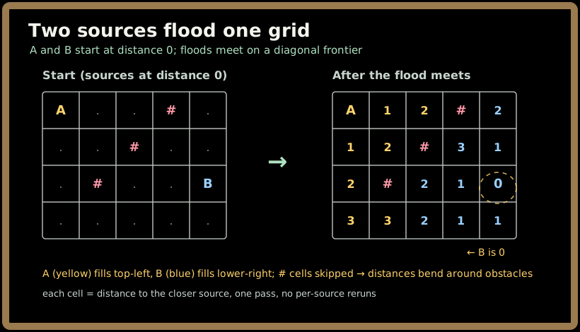
A's wavefront fills the top-left, B's fills the lower-right, and they meet along a diagonal frontier. Each cell holds its distance to the closer of the two — computed in a single pass, no per-source reruns. The # cells are skipped entirely, so distances bend around obstacles for free.

5. Problems in this chapter

▶ Walls and Gates

Fill every empty room in a grid with its distance to the nearest gate, with walls blocking paths. Seed the queue with all gates at once, flood outward, and write each room's distance the first time it's reached. The INF sentinel doubles as the visited check, and the grid is updated in place.
Pattern: multi-source BFS, in-place distance fill. Target: O(rows · cols) time, O(rows · cols) space.

Same pattern, sibling problems: Rotting Oranges (seed all rotten oranges, count rings until every fresh one is reached) and 01-Matrix (seed all 0s, label each 1 with its distance to the nearest 0) are the identical seeded-frontier algorithm — recognise one and you've solved all three.

6. Common pitfalls 🚫

• Running a separate BFS per source. The classic mistake: one BFS from each gate/source, taking minimums. Correct but O(sources · cells). Seed all sources into one queue instead.
• Marking visited too late (on dequeue instead of on enqueue). The same cell gets queued by multiple frontier cells, doing redundant work and, in spread problems, miscounting rings.
• Using min updates and re-queuing. If you've seeded all sources, the first touch is already the minimum — adding min checks and re-enqueues means you've quietly reverted to the per-source mindset.
• Forgetting the empty-source case. No sources → the queue starts empty → BFS does nothing → unreachable cells correctly keep their sentinel. Don't special-case it into a bug.
• Confusing "first reached" with "needs fixing later." Because BFS expands in distance order, a cell's first label is final. There's never a reason to walk back and lower it.

7. Key takeaways

1. Seed every source at distance 0, then run plain BFS. That one move turns "nearest of many" / "spread from many" into a single O(cells) sweep.
2. The virtual super-source is the why: connecting all sources to one free node makes nearest-source distance a plain shortest path — so one BFS suffices.
3. First touch is final. BFS fills cells in distance order; the first frontier to reach a cell gives its minimum. No minimums, no revisits.
4. Mark visited on enqueue and write in place — the cell's own value (sentinel vs filled) is your visited flag and your result at once.
5. It generalises instantly. Walls and Gates, Rotting Oranges, and 01-Matrix are the same algorithm with different seeds and read-outs — which is exactly why interviewers reach for this family to test whether you see the shared structure.