Graph Fundamentals
What is this?
This is the vocabulary chapter — the words you need before anything else makes sense. A graph is just dots (called vertices) joined by lines (called edges), like a subway map where stations are dots and tracks are lines. Once you can describe a graph — is it one-way or two-way? do the lines have lengths? does it loop back on itself? — you can pick the right tool for any graph problem.
💡 Fun fact: the word "graph" here has nothing to do with the bar charts you drew in school. It comes from the Latin "graphicus" by way of mathematician James Joseph Sylvester, who in 1878 borrowed the term to describe chemical-molecule diagrams — atoms as dots, bonds as lines.
🔓 The problem in this chapter is free. Sign in with Google or Microsoft to start solving.
The one-line idea: every graph algorithm is really a question about a property — is it acyclic? is it connected? is it weighted? — so the fastest way to solve graph problems is to fluently read those properties off a graph and map each one to the algorithm it implies. This chapter is that vocabulary.
1. The vocabulary
A graph is G = (V, E) — a set of vertices and a set of edges connecting them. Everything below is a property you observe or impose on that pair.
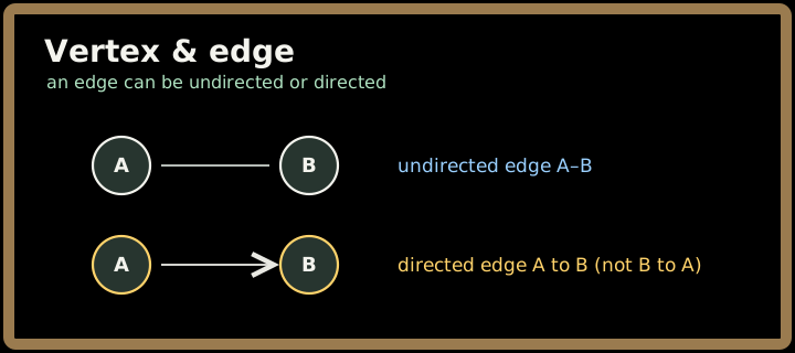
Vertex & edge. A vertex (node) is an entity; an edge is a connection between two of them. An edge may be directed (u → v, one-way) or undirected (u — v, mutual).
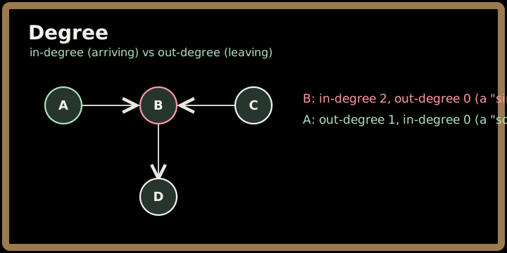
Degree. The number of edges touching a vertex. In a directed graph it splits into in-degree (edges arriving) and out-degree (edges leaving).
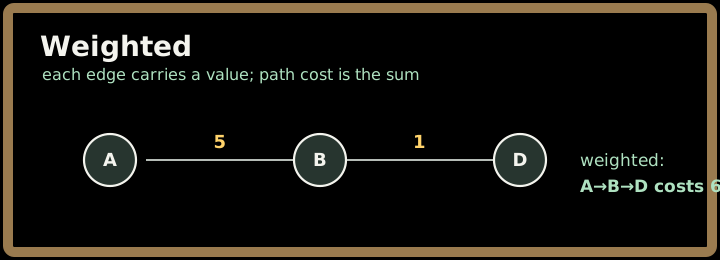
Path. A sequence of vertices each joined to the next by an edge: A → B → D is a path from A to D.
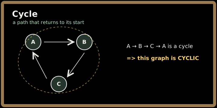
Cycle. A path that returns to its start. A graph with no cycle is acyclic.
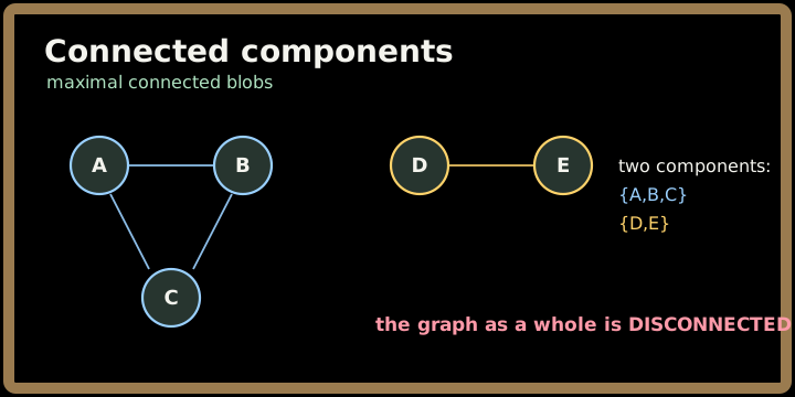
Connected & connected component. An undirected graph is connected if there's a path between every pair of vertices. Otherwise it breaks into connected components — maximal connected blobs.
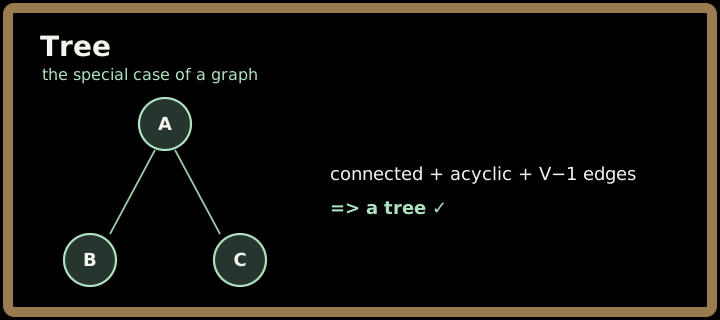
Tree vs general graph. A tree is a connected, acyclic, undirected graph — it has exactly V − 1 edges and a unique path between any two vertices. Add one more edge and you create a cycle; remove one and it disconnects.
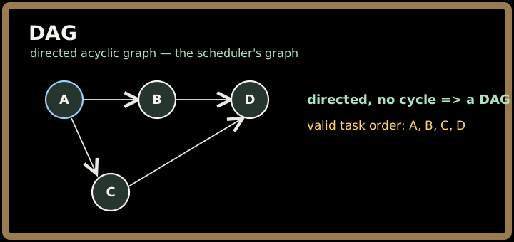
DAG. A Directed Acyclic Graph — directed edges, no directed cycle. The shape of every dependency/scheduling problem; it's exactly the class of graphs you can topologically order.
Dense vs sparse. Dense ≈ E close to its maximum (~V²); sparse ≈ E far below that (often ~V). This single judgement drives your representation choice (matrix vs list).
Weighted. Each edge carries a value — distance, cost, capacity, time. Unweighted graphs treat every edge as cost 1.
2. Where the fundamentals bite in real systems
These aren't textbook labels — each property is a real engineering question:
- Cyclic vs acyclic. A build system, a Terraform plan, a Spark job, an
importgraph — all must be DAGs. A cycle is a bug: a dependency that can never be satisfied. Detecting it is a production correctness check. - Connected components. "Which microservices form an isolated island after this network partition?" "Which user accounts belong to the same fraud ring?" — both are component-finding.
- Degree / centrality. A node with huge in-degree is a hot dependency or a single point of failure; out-degree spikes flag fan-out load.
- Dense vs sparse. A road network is sparse (a city touches a handful of neighbours); a fully-meshed cluster is dense. The judgement decides whether an adjacency matrix is affordable.
- Weighted. Latency, bandwidth, and dollar cost are edge weights — shortest-path over them is literally how routing and logistics work.
3. The fundamentals toolkit — property → algorithm
Reading a property tells you which tool to grab:
| You observe / need… | Reach for… |
|---|---|
| "Is it acyclic? give an order" | Topological sort (Kahn / DFS post-order) |
| "How many groups / islands?" | Connected components via DFS/BFS flood |
| "Are these two connected now?" (dynamic) | Union-Find (DSU) |
| "Shortest path, edges all equal" | BFS |
| "Shortest path, weighted ≥ 0" | Dijkstra |
| "Shortest path, negative edges" | Bellman–Ford (+ negative-cycle detection) |
| "Cheapest connecting edge set" | MST — Kruskal / Prim |
| "Can it be 2-coloured?" | Bipartite check (BFS/DFS alternating) |
| "Visit / reach everything" | DFS or BFS, O(V + E) |
The meta-skill: classify the graph's properties first, and the algorithm is usually a lookup, not an invention.
4. A 30-second worked example
Classify this graph given its edges: 1→2, 2→3, 3→1, 4→3.
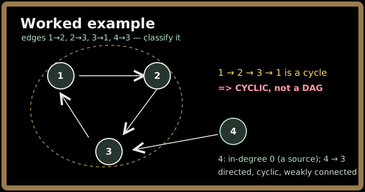
Walk the three questions:
- Directed? Yes — every edge has an arrow.
- Cyclic? Yes —
1 → 2 → 3 → 1returns to its start. So it is not a DAG, and topological sort is impossible here. (If this were a build graph, that 1-2-3 loop is an unresolvable dependency cycle.) - Connected? Treating direction loosely (weakly connected), vertex 4 reaches the rest, so all four hang together. But note 4 has in-degree 0 — nothing points to it; it's a pure source.
Conclusion: a directed, cyclic, weakly-connected graph — fix or break the 1-2-3 cycle and it becomes a DAG you could schedule. That four-second classification is exactly what tells you which algorithm is even applicable.
5. Common pitfalls 🚫
- Directed ≠ undirected. "Connected" and "cycle" mean different things with arrows.
A → Bdoes not let you walkB → A. Mixing this up corrupts both traversal and cycle logic. - Tree assumptions on a general graph. A general graph can have cycles and multiple paths, so you must track visited — without it, traversal loops forever. Trees let you skip that; graphs never do.
- Forgetting disconnected components. A single DFS/BFS from one start only covers that node's component. To process the whole graph, loop over all vertices and launch a traversal from each unvisited one.
- 0- vs 1-indexed vertices. Off-by-one between vertex labels and array indices is the silent killer of otherwise-correct code.
- "Acyclic" without checking direction. An undirected graph with a back-edge has a cycle; a directed graph needs a directed cycle (three-colour DFS), not merely a repeated vertex.
6. Key takeaways
- A graph is V + E, and four properties — directed?, weighted?, cyclic?, connected? — determine everything that follows.
- Each property maps to an algorithm: acyclic ⇒ topological sort, components ⇒ Union-Find/flood, shortest ⇒ BFS (unweighted) or Dijkstra (weighted). Classify, then pick.
- A tree is the special case — connected, acyclic,
V − 1edges, unique paths; general graphs have cycles and demand visited tracking. - A DAG is the scheduler's graph — directed and acyclic is exactly the class you can topologically order.
- Dense vs sparse is the judgement that drives representation (matrix vs list); weighted vs unweighted drives shortest-path choice.
- Spend the first 30 seconds classifying the graph — it tells you which tools are even applicable and prevents applying an algorithm to a graph that violates its assumptions.
Graph Representation
The one-line idea: before you can run a single graph algorithm you must store the graph, and that choice quietly fixes your complexity. Pick the representation that matches your graph's density and the operation you do most — adjacency list for sparse-and-traverse (the interview default), adjacency matrix for dense-and-lookup, edge list for "just give me all the edges."
1. The three representations (one example graph)
We'll store the same small undirected graph in all three forms so you can compare them directly. Label the vertices 0..3:
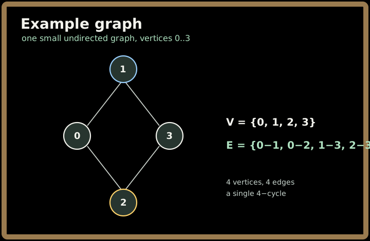
A. Adjacency List — the default
Each vertex maps to a list of its neighbours. Space is exactly proportional to what's actually there: O(V + E).
![Adjacency list mapping each vertex to its neighbours: 0 to [1,2], 1 to [0,3], 2 to [0,3], 3 to [1,2]](https://maangioassets.blob.core.windows.net/diagrams/coding-interview/101/chapters/graph/Graph_Representation_Tutorial-diagram-2.svg)
from collections import defaultdict

# Adjacency list: vertex -> list of neighbours
adj = defaultdict(list)
edges = [(0, 1), (0, 2), (1, 3), (2, 3)]
for u, v in edges:
    adj[u].append(v)
    adj[v].append(u)   # undirected: record BOTH directions
# adj == {0:[1,2], 1:[0,3], 2:[0,3], 3:[1,2]}
Use it when the graph is sparse (E far below V²) and your hot operation is "iterate the neighbours of u" — which is exactly what DFS, BFS, Dijkstra, and topological sort do. This is the right answer ~90% of the time in interviews.
B. Adjacency Matrix
A V × V grid where M[u][v] = 1 (or the weight) marks an edge. Space is O(V²) regardless of how few edges exist.
     0  1  2  3
  0 [ 0  1  1  0 ]
  1 [ 1  0  0  1 ]
  2 [ 1  0  0  1 ]
  3 [ 0  1  1  0 ]
V = 4
M = [[0] * V for _ in range(V)]   # V x V grid of zeros
for u, v in edges:
    M[u][v] = 1
    M[v][u] = 1                   # undirected: symmetric matrix
# "is u–v an edge?"  ->  M[u][v]   in O(1)
Use it when the graph is dense (E ≈ V²), when you need O(1) "is u–v adjacent?" lookups, or for matrix-flavoured algorithms (Floyd–Warshall all-pairs shortest path). Beware: on a sparse graph it wastes memory and makes neighbour iteration O(V) instead of O(degree).
C. Edge List
Just the raw list of edges — no per-vertex indexing at all.
[(0, 1), (0, 2), (1, 3), (2, 3)]
edge_list = [(0, 1), (0, 2), (1, 3), (2, 3)] # (and weights: (u, v, w))
Use it when the algorithm wants to process every edge, order-independent: Kruskal's MST (sort edges by weight) and Bellman–Ford (relax all edges V−1 times) consume edge lists directly. It's also the format most problems hand you the input in — usually your first move is to convert it into an adjacency list.
Sign in to continue reading
The rest of this lesson is available with a free account. Signing in with Google or Microsoft is free.
Sign in to read the full lesson