Connected Components
What is this?
Picture a map of islands in the sea. Each island is a clump of land you can walk across without getting your feet wet, and the open water keeps the islands apart. A "connected component" is exactly one of those islands — a clump where everything is reachable from everything else inside it. This chapter is about a single move: pour water onto one island to flood-mark all of it, then count how many separate floods it takes to cover the whole map. That count is your answer.
💡 Fun fact: the "flood fill" used to mark a component is the same algorithm behind the paint-bucket tool in every image editor — click inside a shape and it spreads color to every connected pixel of the same shade, stopping exactly at the borders, just like flooding one island and no more.
🔓 The 4 problems in this chapter are free. Sign in with Google or Microsoft to start solving.
The one-line idea: A huge family of graph and grid problems reduce to one move — find the disjoint clumps. A connected component is a maximal set of nodes you can reach from one another. Once you see that islands, landmasses, provinces, clusters, and partitions are all just connected components, a single reflex solves them all: flood one component completely, then count (or measure) how many floods it took.
1. What "connected components" really means
A graph splits into components — clusters where every node is reachable from every other node within the cluster, and no edges cross between clusters. Counting them, sizing them, or labelling them is the entire job of this chapter.
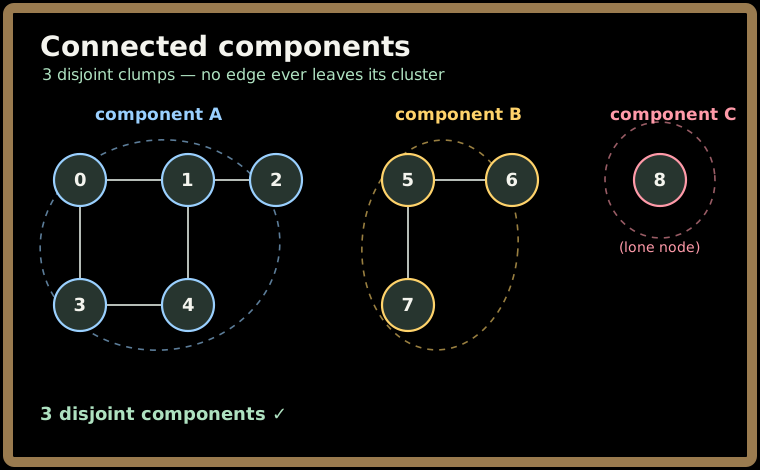
The flood-fill mental model. Pick any unvisited node, then spread outward to every node reachable from it, painting each one "visited" as you go. When the spread stalls, you've painted exactly one component. Resume scanning for the next unpainted node; each fresh start is a new component. That spread is flood fill — DFS or BFS, your pick.
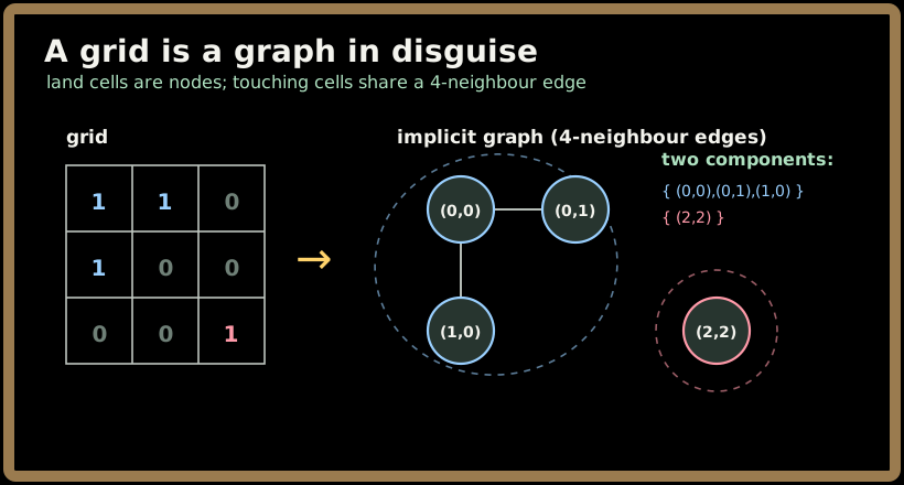
A grid is a graph in disguise. In the island problems there's no explicit edge list. The grid implies one: every land cell is a node, and two land cells are adjacent when they touch up/down/left/right. So "count the islands" is literally "count the connected components of the implicit land-graph."
⚠️ The classic trap: counting nodes instead of components. Summing the
1s in a grid, or1s in a matrix, ignores connectivity. The fix is always the same — flood each clump so it's counted exactly once.
2. Where you'll actually meet this
Connected components are a load-bearing primitive across systems:
- Distributed systems. After a network partition, a reachability matrix splits nodes into groups. Counting components = counting isolated partitions; sizing the largest = finding the group that may still hold quorum and stay writable.
- Image processing / vision. Connected-component labelling: counting cells, defects on a wafer, or objects in a segmented frame; largest-blob analysis for the dominant region.
- Social & recommendation graphs. Community detection — disjoint clusters of users joined by "follows" or "co-purchased" edges.
- Networking. Counting disjoint segments a topology fractured into after link failures; sizing the biggest still-connected segment to route critical traffic.
- Finance / retail / logistics. Grouping accounts by transaction links, warehouses by shared routes, or hubs into independent distribution regions.
Different domains, one question: how many disjoint clumps, and how big are they?
3. The connected-components toolkit
- Flood fill (DFS or BFS). From a seed node, visit everything reachable, marking visited. DFS is shortest to write (recursion or an explicit stack); BFS uses a queue and avoids recursion-depth limits on huge inputs. Both are O(V+E) — for a grid, O(rows·cols).
- Grid → implicit graph. Map a cell
(r,c)to its neighbours. 4-directional[(1,0),(-1,0),(0,1),(0,-1)]for edge-adjacency; add the four diagonals for 8-directional. Always bound-check each neighbour before stepping. - Mark visited — or sink cells. Mutating a grid cell to
0("sinking" it) marks visited in O(1) extra space. If you can't mutate the input, carry avisitedset/array. Forgetting this causes infinite loops and overcounting. - Union-Find (DSU) for counting. Start with
Vcomponents; union the two endpoints of every edge; each successful merge drops the count by one. Near-O(1) per op with path compression + union by rank. The natural choice when edges arrive dynamically or the input is an edge list. - Pick the right fold. The traversal is fixed; only the accumulator changes —
count += 1per flood (count components),max(best, flood_size)(largest component), or stamp a label per cell (label components).
4. A 30-second worked example
Count the islands in this grid by flooding, in one sweep:
1 1 0 1                scan row by row, left to right
0 1 0 1
0 0 0 0
1 0 1 1
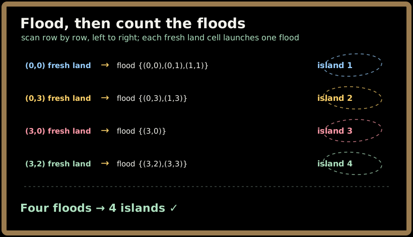
Four floods → 4 islands. Each cell was painted by exactly one flood; every other land cell was already visited when the sweep reached it. That "flood, then count floods" loop is the whole chapter in one move.
5. Problems in this chapter
▶ Number of Islands
Count distinct landmasses in a binary grid under 4-directional adjacency. Sweep the grid; each fresh land cell launches one flood that sinks its whole island; the number of floods is the answer.
Pattern: flood-fill on an implicit grid-graph (DFS / BFS / Union-Find). Target: O(m·n) time, O(min(m,n))–O(m·n) space.
▶ Max Area of Island
Same grid, but report the size of the largest connected landmass. Identical flood-fill — only the accumulator changes: each flood returns its cell count and you keep a running max.
Pattern: flood-fill with an area fold. Target: O(m·n) time.
▶ Number of Provinces
Connected components again, but the graph arrives as a symmetric adjacency matrix. A node's neighbours are a matrix row instead of grid steps. Flood each component (DFS/BFS) or union every edge (Union-Find) and count.
Pattern: connected components on an explicit matrix-graph. Target: O(n²) time, O(n) space.
The throughline: all three are the same algorithm. Only the neighbour function (grid steps vs. matrix row) and the fold (count vs. measure) differ.
6. Common pitfalls 🚫
- Counting nodes, not components. Summing
1s answers the wrong question — you must collapse each connected clump to one count via a flood. - Forgetting to mark visited. Without sinking cells or a
visitedset, flood fill loops forever and recounts cells — the #1 bug. - Marking on dequeue in BFS. Mark a cell visited when you enqueue it, not when you pop it, or the same cell gets queued multiple times.
- Wrong neighbour set. Mixing up 4- vs 8-directional, or missing a bound-check, silently merges or splits components.
- DFS recursion overflow. A near-solid 300×300 grid can blow Python's recursion limit — switch to BFS or an explicit stack.
- Ignoring the gift of structure. For Provinces, the matrix is symmetric with a
1-diagonal — scan only the upper triangle and skip self-loops.
7. Key takeaways
- Connected components are the unifying lens. Islands, landmasses, and provinces are all "find the disjoint clumps."
- Flood, then count (or measure) the floods. Each fresh seed starts exactly one component because the flood paints the rest visited.
- A grid is an implicit graph — cells are nodes, 4/8-neighbour adjacency gives edges; no explicit edge list needed.
- Three interchangeable engines: DFS (shortest), BFS (recursion-safe), Union-Find (best for dynamic edges / edge-list input) — all O(V+E) / O(m·n).
- The traversal is fixed; the fold varies. Swap
count += 1formax(best, size)or per-cell labelling and the same code counts, sizes, or labels components. - Why interviewers lean on this family: it mirrors real systems work — partitions, clustering, segmentation, communities — and rewards spotting one pattern beneath many disguises.
Max Area of Island
Core idea: This is Number of Islands with one twist — instead of counting components, you measure the biggest one. Same flood-fill skeleton, but each flood now returns the size of the component it painted, and you keep a running maximum. Flood a component, total its cells, remember the largest.
1. The problem, in a fresh setting
You manage a fleet of autonomous farm drones. Each drone returns a binary survey grid of a field: 1 = healthy-crop cell, 0 = bare soil. A patch of healthy crop is a group of 1 cells connected up/down/left/right (diagonals don't count). Before scheduling a harvest run you need the size of the single largest contiguous patch — that decides which patch the combine visits first. If the field is all soil, the answer is 0.
Formally: given an m x n binary grid, return the maximum number of 1 cells in any 4-directionally connected component, or 0 if there are none.
| Grid | Max area | Which patch |
|---|---|---|
[[1,1,0,0],[1,0,0,1],[0,0,1,1]] |
3 |
top-left (0,0)(0,1)(1,0) ties the bottom-right (1,3)(2,3)(2,2) — both size 3 |
[[0,0],[0,0]] |
0 |
no crop at all |
[[1,1,1],[1,1,1]] |
6 |
one solid patch covering the grid |
Sign in to continue reading
The rest of this lesson is available with a free account. Signing in with Google or Microsoft is free.
Sign in to read the full lesson