Elasticsearch — Part 1: Foundations & Core Concepts

maang.io System Design Series

---

What is this?

Picture the world's largest library, and you're the person at the front desk. Someone walks up and asks: "Which books mention the phrase 'distributed consensus'?" If your only tool is the shelves, you're doomed — you'd have to open every book and skim every page. No librarian works that way. Instead, at the back of every reference book there's an index: an alphabetical list of terms, and next to each term the exact pages it appears on. To answer the question you don't read books — you read the index, jump straight to "distributed consensus," and it hands you the list of hits instantly.

Now scale that idea up. Instead of one book's index, imagine one giant master index across every book in every branch of the library, kept permanently sorted, that can answer "who mentions X?" in milliseconds — and can also rank the answers by how relevant each book is, not just whether it matched. That master index is what Elasticsearch builds and serves. It is a distributed search and analytics engine that turns "search my data" from a slow scan into an instant lookup.

The one-line idea: A normal database is organized to answer "give me the row with this id"; Elasticsearch flips the data inside-out into an inverted index — organized to answer "give me every document that contains this term, ranked by relevance" — and then spreads that index across a cluster so it stays fast as the data grows.

We'll carry this library analogy — the index at the back of the book, the branches, the head librarian — all the way through to the interview chapter.

---

1. Why Elasticsearch exists — the pain before it

Relational databases are brilliant at structured lookups: WHERE user_id = 42. But ask a SQL database "find every product review that mentions 'battery life' but not 'charger', ranked by how relevant each review is, and while you're at it tell me the top 10 brands by average rating" and it falls apart. Here's why:

• LIKE '%battery%' can't use a normal index. A B-tree index (see the SQL & Data Modeling topic) is sorted by value from the left, so it can find prefixes but not a substring in the middle of a big text blob. A leading-wildcard LIKE degrades to a full table scan — read every row, every time.
• No relevance ranking. SQL gives you rows that match or don't. It has no built-in notion that a review with "battery" in the title, mentioned five times, is more relevant than one that mentions it once in a footnote.
• No linguistic understanding. A user searching "running" probably also wants "run" and "ran"; someone typing "colour" wants "color". Raw SQL matching is literal.
• Analytics on the same box hurt. Slicing "top brands by rating" is an aggregation over the whole dataset, and running it next to your transactional traffic contends for the same resources.

Elasticsearch was built to make all of that fast: full-text search with relevance ranking, language-aware matching, and real-time analytical aggregations — over billions of documents, spread across many machines. It sits on top of Apache Lucene, the battle-tested Java search library that actually implements the inverted index (there's a dedicated Apache Lucene topic in this tier — read it to see the file formats up close). Elasticsearch's own contribution is everything around Lucene: distribution, replication, a REST/JSON API, and a cluster that heals itself.

💡 The rule of thumb people reach for: use your database as the source of truth, and use Elasticsearch as the search and analytics layer you feed from it. We'll defend exactly why at the end of this chapter and again in Part 4.

---

2. The core vocabulary — your mental model

Elasticsearch has its own words. Map them once and everything else clicks.

• Document — the basic unit, a JSON object. One product, one log line, one order. Think: one book in the library.
• Index — a named collection of documents that share a similar shape (e.g. products, logs-2026-07). Not to be confused with the inverted index below — an Elasticsearch "index" is more like a database table (or a library branch). This name collision trips everyone up once; note it and move on.
• Mapping — the schema for an index: which fields exist and their types (text, keyword, integer, date, geo_point…). It tells Elasticsearch how to analyze and store each field. You can let it be inferred (dynamic mapping) or define it explicitly.
• Field — a key in the document. Crucially, a text field is broken into searchable terms (analyzed), while a keyword field is stored whole for exact-match/sorting/aggregation. Same string, two very different behaviors.
• Inverted index — the data structure at the heart of it all: a map from term → list of documents containing that term (the "posting list"). This is the book-index-at-the-back, and it's what makes search fast. We take it apart in Part 2.
• Shard — an index is split into shards so it can outgrow one machine. Each shard is a complete, self-contained Lucene index. Documents are distributed across shards by hashing. Think: library branches, each with its own local catalog.
• Replica — a copy of a shard on another node, for fault tolerance and extra read throughput. Primary shard + its replicas hold identical data.
• Node / Cluster — a node is one Elasticsearch process (usually one server); a cluster is a set of nodes that coordinate and share shards. The head librarian who takes your question and fans it out to the branches is a coordinating node (Part 3).

Here's the containment hierarchy — burn this into memory, because every internals discussion refers back to it:

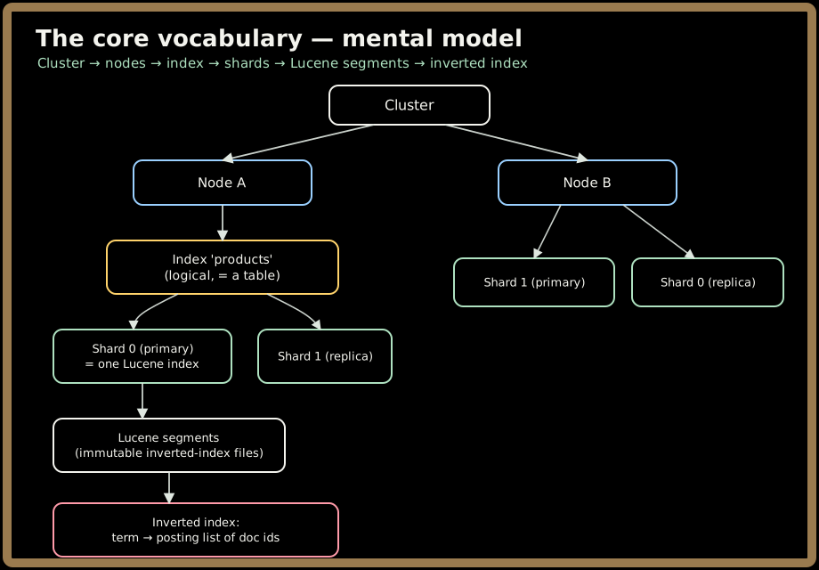
The chain to remember: cluster → nodes → index → shards → Lucene segments → inverted index. A document lives in exactly one primary shard (plus its replicas), and search walks down this chain.

---

3. How you actually use it

Everything is JSON over HTTP. You index a document with a PUT/POST and search with a GET. Here's the whole loop — define a mapping, add a document, run a search:

// 1. Create an index with an explicit mapping
PUT /products
{
  "mappings": {
    "properties": {
      "name":  { "type": "text" },       // analyzed → full-text searchable
      "brand": { "type": "keyword" },    // exact value → filter/aggregate/sort
      "price": { "type": "integer" },
      "created_at": { "type": "date" }
    }
  }
}

// 2. Index a document (the id is optional; ES generates one if omitted)
POST /products/_doc/1
{ "name": "Wireless Noise-Cancelling Headphones", "brand": "Acme", "price": 199 }

// 3. Search: full-text on name, exact filter on brand
GET /products/_search
{
  "query": {
    "bool": {
      "must":   { "match": { "name": "noise cancelling" } },  // relevance-scored
      "filter": { "term":  { "brand": "Acme" } }              // yes/no, no scoring
    }
  }
}

Two things to notice, because they're the whole personality of the query language (the Query DSL):

1. must vs filter. Clauses in must are scored — they contribute to how relevant each hit is (that "noise cancelling" match ranks documents). Clauses in filter are pure yes/no predicates — cheaper, cacheable, and they don't affect the score. Knowing which bucket a clause belongs in is a real performance lever.
2. match vs term. match runs the text through the same analyzer as indexing (lowercasing, splitting into tokens, maybe stemming "cancelling"→"cancel"), so it does language-aware full-text search. term looks for the exact, un-analyzed value — right for that keyword brand field, wrong for free text.

And the other half of Elasticsearch is aggregations — analytics computed on the fly, the "top brands by average price" query SQL made painful:

GET /products/_search
{
  "size": 0,                              // we want stats, not documents
  "aggs": {
    "by_brand": {
      "terms": { "field": "brand" },      // group by brand
      "aggs": { "avg_price": { "avg": { "field": "price" } } }
    }
  }
}

That returns each brand with its average price, computed across the whole cluster in one round trip. Aggregations don't use the inverted index — they use a different, columnar structure called doc values, which we'll meet in Part 3. For now, the takeaway: Elasticsearch is two engines sharing one store — a search engine (inverted index) and an analytics engine (doc values).

---

4. When to reach for it — and when not

Reach for Elasticsearch when the workload has a recognizable shape:

• Full-text search — product catalogs, documentation, code search, "search all my messages" (remember the Cassandra chat app that fanned writes out to Elasticsearch? This is the other side of that).
• Log and observability analytics — the classic ELK/Elastic Stack, where Logstash (or Beats) ships logs in and Kibana visualizes them. Time-stamped, append-mostly, "search and slice recent logs" — read the Logstash topic for the ingestion half.
• Faceted / filtered navigation — the "narrow by brand, price range, rating" sidebars on every e-commerce site, powered by aggregations.
• Real-time-ish analytics dashboards — counts, histograms, percentiles over large datasets, refreshed live.

Be wary — or say no — when:

You need…	Reach for instead
The system of record with strong durability guarantees	A real database (Postgres, Cassandra, DynamoDB) — feed ES from it
ACID transactions, multi-document atomicity	A relational DB; see the Distributed Transactions and Two-Phase Locking topics
Frequent updates to individual records	A database — ES updates rewrite whole documents (Part 2) and churn segments
Relational joins across entities	SQL; in ES you denormalize or use limited parent/child at a cost
Simple key-value by id at massive write rates	Redis, DynamoDB, RocksDB

🚫 The single most common and most dangerous mistake: using Elasticsearch as your primary datastore. It's a superb search layer and a shaky source of truth — its consistency model is near-real-time, not transactional, and reindexing/mapping changes can be painful. If losing the data would be a catastrophe, that data's home is a database, and Elasticsearch is a queryable projection of it. We'll make this concrete in Part 4.

---

5. Key takeaways

1. Elasticsearch is a distributed search and analytics engine over Lucene. Its superpower is the inverted index — data flipped from "row by id" to "term → documents" — which turns full-text search into an instant, ranked lookup instead of a scan.
2. Learn the vocabulary as a hierarchy: cluster → nodes → index (≈ a table) → shards (each a Lucene index) → segments → inverted index. A document lives in one primary shard, replicated for safety.
3. It speaks JSON over HTTP. Master the two halves of the API: the Query DSL (match for full-text/scored, term/filter for exact/cheap) and aggregations (analytics via columnar doc values).
4. Mind the field types: text is analyzed for search, keyword is exact for filtering/sorting/aggregating — same string, opposite behavior.
5. Reach for it for search, logs, and faceted analytics; do not make it your source of truth or your transactional store. Database owns the data; Elasticsearch queries a projection of it.

Next, Part 2 cracks open a single shard: the inverted index in detail, Lucene's immutable segments, and the near-real-time write path — in-memory buffer → refresh → translog → flush → merge — that lets Elasticsearch be both durable and searchable-within-a-second.