Partitioning (Sharding) — Part 1: Foundations & Core Concepts
maang.io System Design Series
What is this?
Imagine you run the national library, and for years every book lived in one enormous building. It worked beautifully — until it didn't. The shelves are full, the front desk is a mob scene, and you physically cannot make the building any taller. You've hit the ceiling of one location.
So you do the only sane thing: you open branch libraries across the city and split the collection among them. No single branch holds everything; each holds a slice. The whole collection still exists — it's just spread out. Add another branch and you get more shelf space and more front desks at once. That is the entire idea of partitioning, also called sharding: take one dataset that's too big or too busy for one machine and split it into pieces, each piece living on a different node.
But splitting immediately raises the only question that matters: when a reader wants a specific book, which branch do you send them to? Get that rule right and every branch stays balanced and findable. Get it wrong and one branch is mobbed while the others gather dust — or worse, nobody can find anything. The whole topic is really about choosing that rule well.
The one-line idea: Partitioning splits one dataset across many nodes so it can grow past the limits of a single machine — and the hard part isn't the splitting, it's choosing the partitioning key and scheme so that data and load land evenly and every request knows exactly which node to ask.
A quick note on words: partition and shard mean the same thing here — one slice of the data living on one node. (Different systems just picked different vocabulary: Cassandra and Kafka say "partition," MongoDB and Elasticsearch say "shard," Postgres says "partition" too.) Throughout this topic I'll say partition and shard interchangeably, exactly as the industry does.
1. Why partitioning exists — the problem it solves
Before partitioning, your options for a growing database were all vertical: buy a bigger machine. More RAM, more CPU, faster disks. This is scaling up, and it works right up until it doesn't:
- A single machine has a hard ceiling. There is a biggest server money can buy, and its price climbs far faster than its capacity. Doubling the box often more-than-doubles the bill.
- One machine is one point of failure. All your eggs, one basket.
- One machine has one set of everything — one disk's worth of throughput, one NIC's worth of network, one CPU's worth of parallelism. A workload that needs more of any of those than one box provides is simply stuck.
Partitioning is scaling out instead: buy ten ordinary machines and split the data across them. Now you have ten disks' worth of I/O, ten NICs' worth of bandwidth, ten CPUs' worth of parallelism — and if one node dies, you've lost a tenth of your capacity, not all of it (and with replication, covered in its own topic, you've lost nothing at all). Ten branches beat one impossibly tall library.
💡 Partitioning is about spreading data and load; replication is about copying data for durability and availability. They're different axes and you almost always use both — you partition to scale, then replicate each partition so a dead node doesn't lose a slice. The rule of thumb: partition for scale, replicate for safety. We'll keep them separate in this topic and lean on the Replication topic for the copying half.
Quick check before moving on:
2. Core concepts and vocabulary
Here's the mental model in five terms. Everything later is built from these.
- Partition / shard — one slice of the dataset, owned by one node. The library branch.
- Partition key — the field whose value decides which partition a record lands in (
user_id,order_id, a timestamp…). This is the design decision. In the library, it's "which property of the book decides its branch" — the author's surname? A hash of the ISBN? The publication year? - Partitioning scheme — the rule that maps a partition key to a partition. The two great families are range and hash (Section 3).
- Rebalancing — moving partitions between nodes when you add or remove capacity, so load stays even. Opening a new branch and shifting some books to it.
- Request routing — the machinery that, given a key, figures out which node currently owns its partition, so a client's request reaches the right place. The library's information desk.
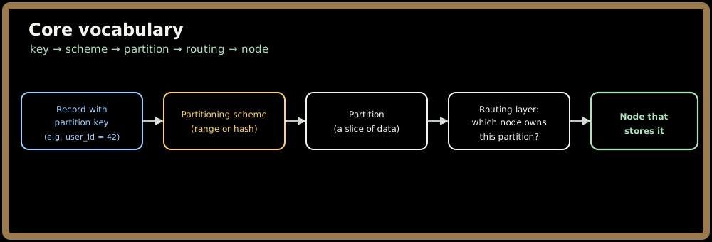
A record's journey is always the same shape: take the partition key → apply the scheme → get a partition → route to the node that owns it. Let's make that concrete.
3. The two great schemes — range vs hash
There are two fundamental ways to map keys to partitions, and the entire trade-off space of partitioning lives in the tension between them. This is the single most important thing to internalize.
3.1 Range partitioning
Range partitioning assigns a contiguous span of key values to each partition. This is the alphabetized library: branch 1 holds authors A–C, branch 2 holds D–F, and so on. Records are kept in sorted order.
- ✅ Range scans are cheap. "Give me every order from Jan 1 to Jan 31" or "every author D through F" touches one partition (or a few adjacent ones) and reads them in order. No fan-out to every node.
- ⚠️ Hotspots are the whole risk. If your key is a timestamp and you're writing now, every single write lands on the one partition holding "recent" — one branch is mobbed while the rest idle. Same if real-world keys clump (everyone's surname starts with S more than X). Range partitioning is only as balanced as your key distribution is uniform, and real data rarely is.
Range partitioning is what powers Bigtable, HBase, and (under the hood) many relational partitioned tables.
3.2 Hash partitioning
Hash partitioning runs the key through a hash function and uses the result to pick a partition. This is the coat-check library: hand over any book, a hash of its title spits out a ticket number, and the ticket says which branch. Similar keys scatter to completely different branches on purpose.
- ✅ Load spreads evenly. A good hash function turns even a clumpy real-world key distribution into a uniform spread across partitions. Sequential IDs, timestamps, popular prefixes — hashing flattens them all. Hotspots from skewed keys mostly vanish.
- ⚠️ You lose range scans. Because adjacent keys are deliberately scattered, "give me Jan 1 through Jan 31" now means asking every partition and merging — a scatter-gather across the whole cluster. Sorted-order queries are gone.
Hash partitioning is the default in Cassandra, DynamoDB, and consistent-hashing systems generally.
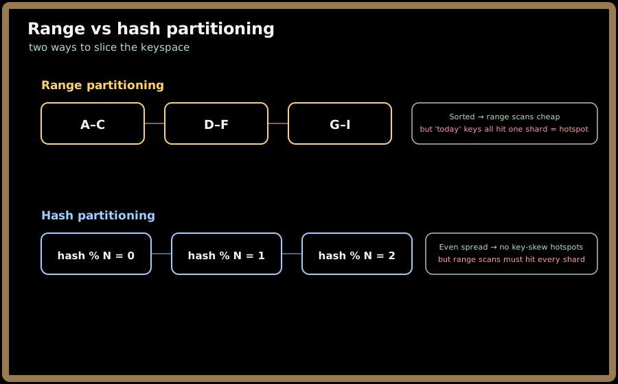
💡 The trade in one sentence: range preserves order (great scans, risky hotspots); hash destroys order (even load, no scans). You cannot have both from a single scheme — choosing between them is the design decision, and it flows directly from your dominant query pattern. Query mostly by ranges of time or key? Range. Query mostly by exact key lookup and fear skew? Hash.
There's a beautiful middle ground: hash the first part of a compound key to pick the partition, then keep the rest sorted within that partition. That's exactly how Cassandra's PRIMARY KEY ((conversation_id), message_id) works — hash on conversation_id for even spread across nodes, sorted on message_id for cheap "latest 50 messages" scans inside one conversation. You get even distribution and local ordering. (See the Apache Cassandra topic — this is its whole data-modeling superpower.)
Quick check before moving on:
4. How you actually use it — a concrete example
You rarely write a hash function by hand; the datastore does it. What you choose is the partition key. Here's the same decision in three flavors so the shape is unmistakable.
Cassandra (hash on the partition key, sorted within it):
CREATE TABLE orders_by_customer (
    customer_id  uuid,       -- partition key: hashed → picks the node
    order_id     timeuuid,   -- clustering key: sorted within the partition
    total        decimal,
    PRIMARY KEY ((customer_id), order_id)
);
-- One customer's orders live together, newest-first. Even spread across nodes.
Postgres (declarative range partitioning by month):
CREATE TABLE events (id bigint, ts timestamptz, payload jsonb)
    PARTITION BY RANGE (ts);
CREATE TABLE events_2026_07 PARTITION OF events
    FOR VALUES FROM ('2026-07-01') TO ('2026-08-01');
-- Queries filtered by ts touch only the relevant month's partition ("partition pruning").
MongoDB (choose hashed vs ranged sharding explicitly):
sh.shardCollection("app.users", { user_id: "hashed" })   // even spread
sh.shardCollection("app.events", { ts: 1 })              // range — beware the "now" hotspot
Notice the pattern: you declare the key and the scheme; the system handles the routing. Your entire job is choosing a key that (a) matches how you'll query and (b) spreads load. Everything in Part 2 is about what the system does underneath that declaration.
5. When to reach for it — and when not
Reach for partitioning when:
- Your dataset or write volume genuinely exceeds what one (replicated) node can hold or serve. This is the real trigger — you've hit the vertical ceiling.
- Your access pattern is friendly to a partition key: you usually query by a single key (→ hash) or by ranges of one key (→ range).
- You need to scale throughput horizontally — more nodes = more parallel capacity.
Think twice — or reach for something else — when:
- Your data fits comfortably on one big replicated box. Then don't shard. Partitioning adds real operational complexity (routing, rebalancing, cross-partition queries, no cheap joins). A single Postgres primary with read replicas serves an astonishing amount of traffic. Premature sharding is a classic over-engineering scar. 🚫
- Your queries constantly span many keys — lots of joins, aggregations across the whole dataset, ad-hoc analytics. Partitioning makes those worse (fan-out to every node). Consider an OLAP/columnar store (Azure Synapse Analytics) or keeping it on one relational box.
- You need multi-partition transactions everywhere. Once a transaction spans partitions you're into Distributed Transactions and Two-Phase Locking (2PL) territory — expensive and complex. If most writes must be transactional across keys, sharding is fighting you.
Alternatives at a glance: vertical scaling (simplest, until the ceiling), read replicas (great for read-heavy, doesn't help write volume or dataset size), caching (the caching topic — shields the DB but doesn't shrink it), and partitioning (the one that actually removes the single-node ceiling). Most mature systems layer all four.
⚠️ The most expensive partitioning mistake isn't a bad scheme — it's sharding too early, before you needed to, and paying the complexity tax for years while a single node would have done fine. And the second most expensive is picking a partition key you can't change later without re-sharding the whole dataset. Choose the key as if you're stuck with it, because you nearly are.
Test yourself on this part's key ideas:
6. Key takeaways
- Partitioning (sharding) splits one dataset across many nodes so it can scale past a single machine's ceiling — more disk, network, and CPU in parallel. It's the scale axis; replication is the separate safety axis, and you use both.
- The partition key + scheme is the whole game. A record's path is always key → scheme → partition → route to owning node.
- Range keeps keys sorted → cheap range scans but hotspot-prone if keys clump (especially timestamps). Hash scatters keys → even load but no range scans. You pick based on your dominant query pattern; you can't get both from one scheme.
- A compound key (hash the partition part, sort within it) gives you even spread and local ordering — the trick behind Cassandra-style modeling.
- Don't shard until you must. If the data fits on one big replicated box, that's simpler and cheaper. And choose the partition key carefully — you're effectively stuck with it.
Next, Part 2 goes under the hood: how the routing layer actually finds a partition, why hash % N is a rebalancing trap (and what real systems do instead), how partitions split and move, how to tame a hot key, and how secondary indexes get partitioned two very different ways.