SQL & Data Modeling — Part 1: Foundations & Core Concepts

maang.io System Design Series

---

What is this?

Picture a well-run town library. Every book has a single index card in a drawer, and that card lives in exactly one place, filed by a unique call number. When the library buys a new copy, it doesn't rewrite the author's full biography onto every card — it keeps one author card and points the book cards at it. Want everything by a given author? You pull the author card, follow the pointers, and gather their books. Want to find a book fast among two million of them? You don't walk the shelves — you flip through the sorted catalog drawer, which lets you jump straight to the right card.

That library is a relational database, and the discipline of laying out those cards and pointers so that every fact is stored once, cleanly, and can be found fast is data modeling. SQL (Structured Query Language) is the language you use to ask the librarian questions: "give me every book by this author published after 2010, sorted by title." You describe what you want; the database figures out how to fetch it.

The one-line idea: the relational model stores your data as a set of tables (relations) linked by keys, and good data modeling means arranging those tables so that each fact lives in exactly one place — which makes updates safe, storage lean, and queries composable, at the cost of having to join things back together at read time.

We'll carry this library through all three chapters: relations are the drawers of cards, keys are the call numbers and cross-reference pointers, and later — in Part 2 — the sorted catalog drawer becomes the B+tree index and pulling matching cards from two drawers becomes a join algorithm.

---

1. Why the relational model exists — the pain before it

Before relational databases, applications stored data in bespoke file formats and navigational databases where the access path was baked into the data. If you'd wired records together as "each order points to the next order for this customer," then answering a question the original designer hadn't anticipated — "which products did customers in Ohio buy last March?" — meant writing new traversal code, sometimes reorganizing the files. Data and access were fused.

In 1970, Edgar Codd's relational model made a radical split: store data as plain tables of facts, and let a general-purpose query language derive any view you want on demand. You no longer navigated pointers by hand; you declared a query and the system computed the answer. Two consequences that still define the model today:

• Data independence. The logical shape of your data (tables and columns) is decoupled from how it's physically stored and indexed. You can add an index, change the storage engine, or reorganize files without rewriting a single query.
• Declarative querying. You say what (SELECT name FROM customers WHERE state = 'OH'), not how (loop, seek, merge). A query planner — the subject of Part 2 — turns the what into an efficient how.

That flexibility is exactly what a naive "just duplicate the data wherever it's convenient" approach destroys, which brings us to the central skill.

---

2. Core concepts & vocabulary — the mental model

2.1 Relations, tuples, attributes

A relation is a table: a set of rows over a fixed set of typed columns. The formal words are worth knowing because interviewers use them:

• Relation = the table (customers).
• Tuple = one row (one customer).
• Attribute = one column (email).
• Domain = the type/allowed values of an attribute (email is text; age is a non-negative integer).

A relation is a set of tuples — order doesn't matter and there are no duplicate rows (a proper key guarantees that). "Set-based thinking" is why SQL operates on whole result sets at once rather than row-by-row loops.

2.2 Keys — the call numbers and cross-references

Keys are how the model keeps rows identifiable and tables linked. Five terms, each building on the last:

• Super key — any set of columns that uniquely identifies a row (possibly with extra, unnecessary columns). {customer_id, email, name} is a super key if customer_id alone already identifies the row.
• Candidate key — a minimal super key: no column can be removed without losing uniqueness. A table can have several. For a customer, both customer_id and email might be candidate keys.
• Primary key (PK) — the one candidate key you choose as the row's official identity. It's non-null and unique, and it's usually what other tables reference. In our library, it's the call number.
• Foreign key (FK) — a column in one table that references the primary key of another, wiring the two together. orders.customer_id is an FK pointing at customers.customer_id — the "this book was written by that author" pointer. The database can enforce it (referential integrity): you can't insert an order for a customer who doesn't exist, and depending on the rule you can't delete a customer who still has orders.
• Composite key — a key made of more than one column, e.g. an order_items table keyed on (order_id, product_id) because a line item is identified by which order and which product together.

💡 A primary key is a choice, not a fact. When several candidate keys exist (say email and a numeric id), prefer a stable, narrow, meaningless surrogate key (an auto-generated id) as the PK, because natural keys like email change and cascade that change through every foreign key. This is a real modeling decision, not pedantry.

2.3 The whole picture — an ER model

Before you write any CREATE TABLE, you sketch an entity-relationship (ER) model: the entities (nouns your system cares about — customers, orders, products), their attributes, and the relationships between them (a customer places many orders; an order contains many products). Here's a small e-commerce model:

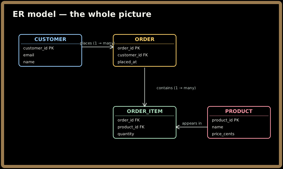
Read the crow's-foot notation as cardinality: ||--o{ means "one customer places zero-or-many orders." The ORDER_ITEM table in the middle resolves the many-to-many relationship between orders and products — a classic modeling move called a junction (or associative) table, keyed on the composite (order_id, product_id).

---

3. Normalization — putting each fact in exactly one place

Here's the failure the whole discipline exists to prevent. Imagine you got lazy and crammed everything into one wide table:

-- The anti-pattern: one big flat table
orders_flat(order_id, customer_email, customer_name, customer_address,
            product_name, product_price, quantity, placed_at)

Every row repeats the customer's name and address and the product's name and price. This one table has three anomalies that will bite you in production:

• Update anomaly. A customer moves. Their address appears on 400 order rows. Update 399 and miss one → the same customer now has two "true" addresses and your data is silently corrupt.
• Insertion anomaly. You want to add a new customer who hasn't ordered yet — but there's no row to put them in without inventing a fake order. The design forces unrelated facts to co-exist.
• Deletion anomaly. You delete the last order for a customer → you accidentally erase the only copy of that customer's address. Deleting one fact destroys another.

The cure is normalization: a sequence of increasingly strict rules (normal forms) that progressively split tables so each fact lives once. Walk them in order:

Normal form	The rule, plainly	What it removes
1NF — First	Every column holds a single atomic value; no repeating groups or comma-lists in a cell, no arrays-as-a-column. Each row is unique (has a key).	"Multiple products crammed into one products cell."
2NF — Second	1NF and every non-key column depends on the whole composite key, not just part of it. (Only relevant when the key is composite.)	Partial dependency — e.g. product_name in order_items(order_id, product_id, product_name) depends only on product_id, not the whole key.
3NF — Third	2NF and no non-key column depends on another non-key column.	Transitive dependency — e.g. storing customer_city alongside customer_zip when city is determined by zip.
BCNF — Boyce-Codd	3NF and every determinant (anything that determines other columns) is a candidate key. A stricter 3NF that closes rare edge cases with overlapping candidate keys.	The last "a non-key determines a key-part" anomalies 3NF can miss.

💡 The pragmatic rule of thumb every practitioner actually uses: "the key, the whole key, and nothing but the key." 1NF says facts hinge on a key; 2NF says on the whole key; 3NF says on nothing but the key. Reach 3NF and you've eliminated the vast majority of anomalies. BCNF matters occasionally; 4NF/5NF are rare in interviews.

Normalizing orders_flat to 3NF gives you exactly the four-table model in the ER diagram above: customers, orders, products, and the order_items junction. Now the customer's address lives in one row, in customers. Move? One update. Add a customer with no orders? One clean insert. Delete an order? The customer survives. Every anomaly is gone — because every fact has a single home.

---

4. How you actually use it — a short worked schema and query

Here's the normalized schema and the join that reassembles a customer's order at read time:

CREATE TABLE customers (
    customer_id  BIGSERIAL PRIMARY KEY,
    email        TEXT UNIQUE NOT NULL,
    name         TEXT NOT NULL,
    address      TEXT
);

CREATE TABLE orders (
    order_id     BIGSERIAL PRIMARY KEY,
    customer_id  BIGINT NOT NULL REFERENCES customers(customer_id),
    placed_at    TIMESTAMPTZ NOT NULL DEFAULT now()
);

-- "What did customer 42 order, with product names and totals?"
SELECT o.order_id, p.name, oi.quantity, oi.quantity * p.price_cents AS line_total
FROM   orders o
JOIN   order_items oi ON oi.order_id = o.order_id
JOIN   products p     ON p.product_id = oi.product_id
WHERE  o.customer_id = 42
ORDER  BY o.order_id;

Notice the shape of the deal. Because we split the facts apart to store them safely, we must join them back together to read them. That reassembly — three tables stitched on their keys — is the price of a clean model, and it's what the query planner and join algorithms in Part 2 make fast. The REFERENCES clause is the enforced foreign key: the database itself guarantees no order can point at a non-existent customer.

---

5. When to reach for it — and when not

Reach for a relational database (SQL) when:

• Your data is structured and relationships matter — entities that reference each other, where integrity ("no orphan orders") is worth enforcing.
• You need flexible, ad-hoc queries — you can't predict every question up front, and you want joins, filters, aggregations, and grouping on demand.
• You need real transactions — multiple rows changed atomically with the guarantees from the ACID chapter (all-or-nothing, isolated, durable). Move money, and you want this.
• Data volume is moderate-to-large but fits a well-indexed cluster — millions to low billions of rows, served from a primary with read replicas.

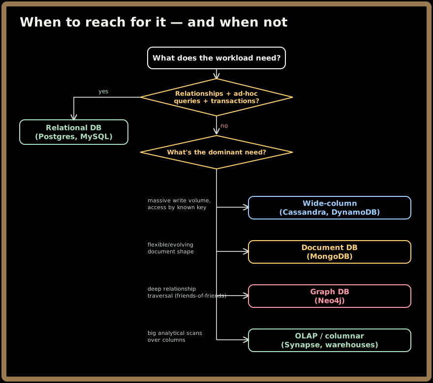
Reach for something else when the workload wants what the relational model traded away — the full comparison is the SQL vs NoSQL topic, but at a glance:

⚠️ The classic footgun is over-normalizing a read-heavy path. A perfectly 3NF schema can turn one screen render into a six-table join executed thousands of times a second. The fix isn't to abandon relational — it's deliberate denormalization (Part 2) where you measure the join cost and choose to duplicate a fact on purpose, with your eyes open. Normalize by default; denormalize as a considered exception.

---

Key takeaways

1. The relational model stores facts as tables (relations) of typed rows (tuples), linked by keys — and separates the logical shape of data from its physical storage, which is what makes declarative, ad-hoc querying possible.
2. Keys are the backbone: a candidate key is a minimal unique identifier, the primary key is the one you elect (prefer a stable surrogate), and foreign keys wire tables together with enforceable referential integrity.
3. Normalization is the craft of putting each fact in exactly one place — 1NF (atomic) → 2NF (whole key) → 3NF (nothing but the key) → BCNF — and it exists to kill the update, insertion, and deletion anomalies that duplication causes.
4. The trade is explicit: you split data apart to store it safely, then join it back to read it. Clean writes now, more work at read time — the mirror image of the denormalize-for-reads bargain we'll make deliberately in Part 2.
5. Reach for SQL when structure, integrity, transactions, and flexible queries matter; reach elsewhere (see the SQL vs NoSQL topic) when the workload's shape wants raw write throughput, schema flexibility, deep graph traversal, or analytical scans instead.

Next, Part 2 goes under the hood: how a B+tree index turns a full-table scan into three page reads, how the query planner chooses between nested-loop, hash, and merge joins, how the write path uses the write-ahead log, and when a Staff engineer deliberately denormalizes — with real numbers.