Azure Synapse Analytics — Part 1: Foundations & Core Concepts

maang.io System Design Series

---

What is this?

Imagine a colossal warehouse that has to answer a single question: "How many blue widgets did we ship to Europe last year?" The answer is buried in a billion shipping records. One clerk with one ledger would be reading for a week. So the warehouse hires a smarter setup: a foreman who reads the question and writes out picking tickets, and a crew of workers who each own a fixed set of numbered bins where the records live. The foreman doesn't touch a single record himself — he splits the question into 60 identical little questions ("count the blue-Europe widgets in your bins"), hands one to each worker, they all count in parallel, and he adds up the 60 partial answers into one number. A week's work finishes in seconds, because sixty people counted at once.

That warehouse is Azure Synapse Analytics — specifically its dedicated SQL pool, a cloud MPP (Massively Parallel Processing) data warehouse. The foreman is the control node, the workers are compute nodes, and the numbered bins are the famous 60 distributions. Everything in this topic comes back to that image: split the data across 60 bins, split the question across the crew, and never make workers carry records to each other's desks if you can avoid it.

The one-line idea: Synapse answers analytical questions over enormous tables by sharding every table into 60 distributions and running one SQL query as 60 parallel sub-queries. The whole game — the whole reason a Staff engineer tunes it — is arranging your data so each worker can answer using only the bins it already owns, avoiding the expensive step of shuffling data between distributions.

Let's build up the mental model, then run a real query.

---

1. Why it exists — the problem before MPP

For decades, analytics meant pointing a query at the same relational database that ran the application — a single, powerful (and eye-wateringly expensive) server. That works until it doesn't. A row-oriented OLTP database like the ones in the SQL & Data Modeling topic is built to fetch one order for one customer in a millisecond. Ask it instead to scan every order across five years and sum a column, and it grinds: it's reading whole rows off disk (including 40 columns you don't want), it can't spread the scan across more than one box, and it's competing with live customer traffic for the same CPU.

The classic fixes all hit a wall:

• Scale up (a bigger single server) — you eventually run out of "bigger," and you're paying for a monster 24/7 to serve a report that runs at 8 a.m.
• Read replicas — help concurrency, but one replica still scans a billion rows on one machine. You haven't parallelized the single query.
• Bolt analytics onto the OLTP box — now your month-end report locks tables and pages the on-call engineer.

MPP is the structural answer: instead of one big machine, use many machines that share nothing — each owns its own slice of the data and its own CPU/memory/disk — and make a single query run on all of them at once. That's the same divide the data, divide the work instinct behind the Partitioning (Sharding) topic, applied to analytical queries. Synapse is Microsoft's managed, cloud-native take on it, descended from the old "SQL Data Warehouse" (SQL DW) product.

💡 The mental split you must keep straight is OLTP vs OLAP. OLTP (Online Transaction Processing) = many tiny reads/writes touching one row — the app database. OLAP (Online Analytical Processing) = few huge queries scanning billions of rows and aggregating — the warehouse. Synapse's dedicated pool is an OLAP engine. Using it for OLTP (single-row lookups, high-frequency updates) is the single most common way people misuse it. More on this in Part 3.

---

2. The core mental model

2.1 Control node + compute nodes (shared-nothing)

A dedicated SQL pool has exactly one control node and one or more compute nodes.

• The control node is the brain (the foreman). It speaks T-SQL to your client, but it stores no user data. It parses the query, runs the cost-based MPP optimizer, and produces a distributed query plan — a set of steps that the compute nodes execute in parallel. It then gathers their partial results and returns the final answer.
• The compute nodes are the muscle (the crew). Each one owns a portion of the data and runs its slice of the plan against its own local storage and CPU. They share nothing — no shared disk, no shared memory — which is exactly why they scale linearly.

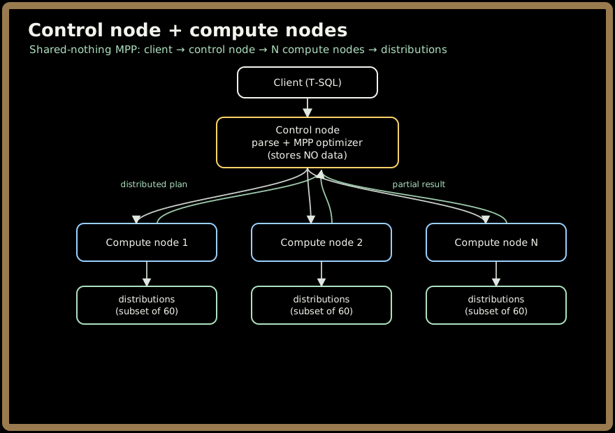
2.2 The 60 distributions — the fixed unit of parallelism

Here's the detail that trips people up and that you must have cold: a dedicated SQL pool always has exactly 60 distributions. Not 59, not 64 — always 60. A distribution is a bucket of storage and the unit of parallel processing: every table you create is physically chopped into 60 pieces, one per distribution.

What changes when you scale is how many compute nodes those 60 distributions are spread across:

• At the smallest size (DW100c), you have 1 compute node that owns all 60 distributions.
• Scale up and the 60 get redistributed: DW1000c → 2 nodes (30 distributions each), DW5000c → 10 nodes (6 each), and at the top (DW30000c) → 60 nodes, one distribution each.

You buy compute in units called DWUs (Data Warehouse Units, sometimes written cDWU for the Gen2 "compute" DWU) — an abstract bundle of CPU, memory, and I/O. Scaling from DW500c to DW1000c roughly doubles your crew.

💡 Why 60? It's a highly composite number — divisible by 1, 2, 3, 4, 5, 6, 10, 12, 15, 20, 30, 60. That means as you scale the node count up, the 60 distributions always divide evenly across the nodes, so no worker is ever stuck with an uneven load. Whatever DWU you pick, the crew splits the bins perfectly.

2.3 Dedicated vs serverless SQL pools

Synapse actually gives you two SQL engines, and choosing wrong is a classic mistake:

	Dedicated SQL pool	Serverless SQL pool
Data lives	Ingested into the pool's managed columnstore	In place in your data lake (Parquet/CSV/Delta on Azure Blob / ADLS)
You pay for	Provisioned DWUs (reserved compute, ~per hour)	Per TB scanned (~pay-as-you-go, no infra)
Scaling	You pick/adjust DWUs; can pause to stop paying compute	Fully elastic, nothing to manage
Best for	Predictable, high-concurrency enterprise data warehouse	Ad-hoc exploration, a "logical" warehouse over the lake

The dedicated pool is the "warehouse with a permanent crew" — you provision it, load data into its own optimized storage, and it's ready for heavy, repeated reporting. The serverless pool is "hire a crew by the hour to read files you already have" — it queries raw files sitting in Object Storage (S3 & Azure Blob) directly with OPENROWSET, charging only for bytes scanned. Most of this topic focuses on the dedicated pool, because that's where the meaty MPP internals — distributions, columnstore, data movement — actually live.

(Both live inside a Synapse workspace, which also bundles Apache Spark pools and data-integration pipelines. Useful to name, but the SQL/MPP engine is the interview substance.)

---

3. How you actually use it

You talk to Synapse in T-SQL — it looks like SQL Server. The interesting part is the extra clause when you CREATE TABLE: you must tell it how to distribute the rows across the 60 buckets. This one decision drives everything in Part 2.

-- A big FACT table: hash-distribute it on the column you'll join/group by.
CREATE TABLE dbo.FactSales
(
    SaleId       BIGINT      NOT NULL,
    CustomerId   BIGINT      NOT NULL,
    ProductId    INT         NOT NULL,
    SaleDate     DATE        NOT NULL,
    Amount       DECIMAL(12,2)
)
WITH
(
    DISTRIBUTION = HASH(CustomerId),      -- which of the 60 bins each row lands in
    CLUSTERED COLUMNSTORE INDEX           -- columnar storage (the default; Part 2)
);

-- A small DIMENSION table: replicate a full copy to every compute node.
CREATE TABLE dbo.DimCustomer
(
    CustomerId   BIGINT NOT NULL,
    Name         NVARCHAR(100),
    Country      NVARCHAR(50)
)
WITH ( DISTRIBUTION = REPLICATE );

Three distribution strategies exist, and choosing between them is the skill:

• HASH(column) — a hash of that column decides the bucket. Same value → same bucket, every time. Use for big fact tables, hashed on the column you most often join or aggregate on.
• ROUND_ROBIN — spray rows evenly across the 60 buckets, next-bucket-each-time, ignoring content. The default. Dead simple, perfectly even, but you have no idea where any given row is — so joins usually need shuffling. Great for staging/load tables.
• REPLICATE — keep a full copy of the whole table on every compute node. Zero shuffle when you join to it. Only sane for small dimension tables (rule of thumb: under ~2 GB).

Once loaded, you query it like any SQL warehouse — a star-schema join between the fact and its dimensions:

SELECT c.Country, SUM(f.Amount) AS Revenue
FROM   dbo.FactSales   f
JOIN   dbo.DimCustomer c ON f.CustomerId = c.CustomerId
WHERE  f.SaleDate >= '2025-01-01'
GROUP BY c.Country;

The control node turns that single statement into a 60-way parallel plan. How well it runs depends almost entirely on whether your distribution choices let each worker answer from its own bins — the subject of Part 2.

---

4. When to reach for it — and when not

Reach for a Synapse dedicated pool when the shape of the problem is:

• A central enterprise data warehouse — many source systems funneled into a star schema for BI dashboards, finance reports, and analysts.
• Huge scans + aggregations — "sum/average/count over billions of rows," where columnar storage and 60-way parallelism shine.
• Predictable, concurrent reporting — a known daily/hourly workload where reserving compute (and pausing it overnight) is cost-effective.

Reach for something else when:

If you need…	Use instead
Single-row lookups, high-frequency updates (OLTP)	Azure SQL DB / Postgres / a row store
Ad-hoc queries over files you already have in the lake	Serverless SQL pool or Spark
Key-value / write-heavy always-on workloads	Apache Cassandra / DynamoDB (the SQL vs NoSQL topic)
Real-time streaming aggregation	Apache Flink / Kafka + a stream processor
Full-text search	Elasticsearch

⚠️ The number-one footgun: treating a dedicated pool like an OLTP database. It has no enforced primary keys, no foreign keys, and no unique constraints (you can declare a PRIMARY KEY NONCLUSTERED NOT ENFORCED, but the engine won't police it). It's built for scanning, not point lookups, and it caps concurrent queries low (tens, not thousands). If your workload is lots of small transactions, you've picked the wrong tool — a mistake we'll make loud in Part 3.

---

5. Key takeaways

1. Synapse (dedicated SQL pool) is a cloud MPP data warehouse: one control node (the brain, no data) plans a query; compute nodes (the muscle) run it in parallel over their own shared-nothing storage.
2. Always exactly 60 distributions. They're the fixed unit of parallelism; scaling (DWUs) changes only how many compute nodes those 60 buckets spread across (1 node owns all 60 at the smallest size; 60 nodes own one each at the largest).
3. Every table declares a distribution: HASH (big facts, aligned to joins), ROUND_ROBIN (even, simple, staging — the default), or REPLICATE (small dimensions copied everywhere). This one choice governs performance.
4. Dedicated vs serverless: dedicated = provisioned compute over ingested columnar storage (the enterprise EDW); serverless = pay-per-TB queries over files sitting in the data lake (ad-hoc).
5. It's OLAP, not OLTP. Reach for it for big scans and aggregations in a star schema; reach for a row store the moment you need point lookups, high-frequency writes, or enforced constraints.

Next, Part 2 opens the warehouse doors: how the 60 distributions physically store data as a clustered columnstore index, what happens on the read and write paths, and the single most important internal cost a Staff engineer must reason about — data movement (shuffles) between distributions.