Quadtree — Part 1: Foundations & Core Concepts

maang.io System Design Series

---

What is this?

Picture a giant paper map of a city pinned to the wall of a dispatch office, and every time a delivery driver comes online you stick a pushpin where they are. For a quiet suburb that's fine — a handful of pins, easy to scan. But downtown at lunchtime, hundreds of pins pile onto the same few square blocks until it's a solid clot of plastic and you can't tell one from another. So you do the obvious human thing: you take that one crowded district, draw a crosshair through its middle, and split it into four smaller districts. If the top-right of those four is still a mess, you split that one into four again. You keep subdividing only where it's crowded, leaving the quiet suburbs as one big undivided square.

That habit — recursively cut a crowded region of the plane into four quarters, and stop when a quarter is calm enough — is a quadtree. The pushpin map is the analogy we'll carry through all three chapters, because it captures the whole idea: the tree isn't uniform, it's deep where the data is dense and shallow where it's sparse, and that's precisely what makes it fast.

The one-line idea: A quadtree recursively subdivides a 2D region into four quadrants — NW, NE, SW, SE — splitting a quadrant only when it holds too many points, so the structure automatically spends its resolution where the data actually is and lets you answer "what's near here?" without scanning everything.

Let's unpack why anyone needed this, then the vocabulary, then how you actually use one.

---

1. The problem: "find things near this point" is brutal without structure

Suppose you have one million driver locations and a rider standing at some (lat, lng). You want every driver within 2 km. The naive answer is a linear scan: compute the distance to all one million drivers and keep the close ones. That's O(n) per query, and you have thousands of riders querying every second. It doesn't scale, and it's obviously wasteful — you're measuring the distance to a driver on the other side of the country to answer a question about your own neighbourhood.

The pain is that a plain database index doesn't help here. A B-tree index (the kind behind WHERE lat BETWEEN ...) sorts on one dimension at a time. You can index latitude, but then a query for "within 2 km" still drags back every driver in a 2 km-tall horizontal band stretching across the entire map, and you re-filter by longitude in memory. Two-dimensional "nearness" is fundamentally not a one-dimensional sort problem, and that mismatch is the whole reason spatial data structures exist.

What we want is a structure where nearby points live near each other in the structure too, so a query can throw away 99% of the world in a few pointer hops and only look closely at the neighbourhood that matters. That's the job of a spatial index, and the quadtree is one of the oldest and most intuitive ways to build one.

---

2. Core concepts & vocabulary — the mental model

A quadtree is a tree where every internal node has exactly four children, one per quadrant of a rectangular region. The names are compass directions:

• NW (north-west, top-left), NE (north-east, top-right), SW (south-west, bottom-left), SE (south-east, bottom-right).

Each node owns an axis-aligned bounding box — the rectangle of the plane it's responsible for. The root owns the whole world; its four children own the four quarters of that world; their children own the sixteenths; and so on. A point at (x, y) belongs to exactly one child at each level — the one whose box contains it — so lookup is just "which quarter am I in?" repeated down the tree.

The single most important tuning knob is node capacity (also called bucket size): the maximum number of points a leaf is allowed to hold before it must split. When you insert a point into a leaf that's already at capacity, the leaf subdivides into four children, its points are re-distributed into those children by position, and the once-leaf becomes an internal node. This is exactly the "downtown got too crowded, cut it into four" move from the pushpin map.

A few more terms you'll meet:

• Leaf node — a node with no children that actually stores points (up to capacity). This is where data lives.
• Internal node — a node that has been split; it stores no points itself (in the common point-region flavour), only four child pointers.
• Depth / height — how many splits deep the tree goes. Crucially, depth is not uniform: dense regions are deep, sparse regions are shallow.

2.1 Three flavours you should be able to name

Interviewers reward you for knowing these aren't all "quadtree" — they're a family:

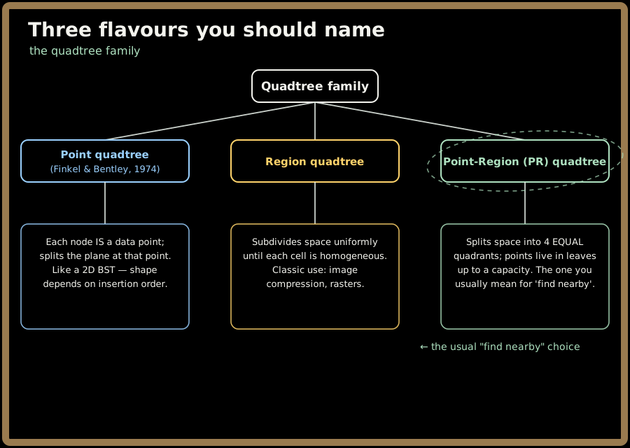
• Point quadtree — the original (Finkel and Bentley, 1974). Each node is one of your data points, and the split lines pass through that point, carving the plane into four unequal quadrants. It behaves like a two-dimensional binary search tree: elegant, but its shape depends on insertion order and deletion is fiddly.
• Region quadtree — subdivides space itself into equal quarters, ignoring the data, and keeps splitting a quadrant until it's "uniform" (e.g. all the same colour in an image). This is the flavour behind image compression and raster/GIS tiling: a big block of blue sky becomes one shallow leaf, while a detailed cityscape becomes deep.
• Point-Region (PR) quadtree — the workhorse for location data and the one we'll implement in Part 2. It splits space into four equal quadrants (like a region quadtree) but stores points in its leaves up to a fixed capacity (like a point quadtree's payload). When you hear "quadtree for find-nearby / maps / collision detection," this is almost always the one people mean. Whenever this series says "the quadtree" without qualification from here on, we mean the PR quadtree.

💡 Rule of thumb: point quadtree = "the node is the data, split at the point." Region/PR quadtree = "split the space into equal quarters, hang the data in the leaves." The equal-quarter split is what makes PR quadtrees easy to reason about and easy to map onto the recursive-bisection encodings you'll meet in the Geohashing topic.

---

3. How you actually use one — a short example

You rarely hand-write a quadtree in an interview, but you should be able to sketch the shape. The two operations that matter are insert and query a region. Here's the skeleton, kept deliberately small:

class QuadTree:
    def __init__(self, boundary, capacity=4):
        self.boundary = boundary      # a rectangle: x, y, w, h
        self.capacity = capacity      # max points before this leaf splits
        self.points = []              # holds points while still a leaf
        self.divided = False          # becomes True after a split
        # children (created lazily on split): nw, ne, sw, se

    def insert(self, point):
        if not self.boundary.contains(point):
            return False              # not my region — reject
        if len(self.points) < self.capacity and not self.divided:
            self.points.append(point) # room in this leaf — done
            return True
        if not self.divided:
            self.subdivide()          # full leaf → cut into 4 equal quads
        # hand the point to whichever child's box contains it
        return (self.nw.insert(point) or self.ne.insert(point)
                or self.sw.insert(point) or self.se.insert(point))

    def query_range(self, area, found):
        if not self.boundary.intersects(area):
            return found              # my box is nowhere near the query — prune
        for p in self.points:
            if area.contains(p):
                found.append(p)
        if self.divided:
            for child in (self.nw, self.ne, self.sw, self.se):
                child.query_range(area, found)
        return found

The whole payoff is in that first line of query_range: if a node's bounding box doesn't intersect your query rectangle, you return immediately and never descend into its subtree. One cheap rectangle-overlap test prunes away an entire quarter of the map — and recursively, a quarter of a quarter, and so on. That's how you answer "drivers within 2 km" while touching only the handful of leaves that actually cover your neighbourhood, instead of all one million points.

---

4. When to reach for it — and when not

A quadtree is the right tool when your data is points (or small objects) in a 2D plane and your queries are "what's inside this box / near this point," especially when the data is unevenly clustered (cities dense, oceans empty) — because the adaptive depth is exactly what handles skew gracefully. Games use it for broad-phase collision detection (only test pairs of objects that share a leaf); maps use it for find-nearby; image tools use the region variant for compression; physics simulators use it in the Barnes–Hut approximation for n-body gravity.

But reach for something else when:

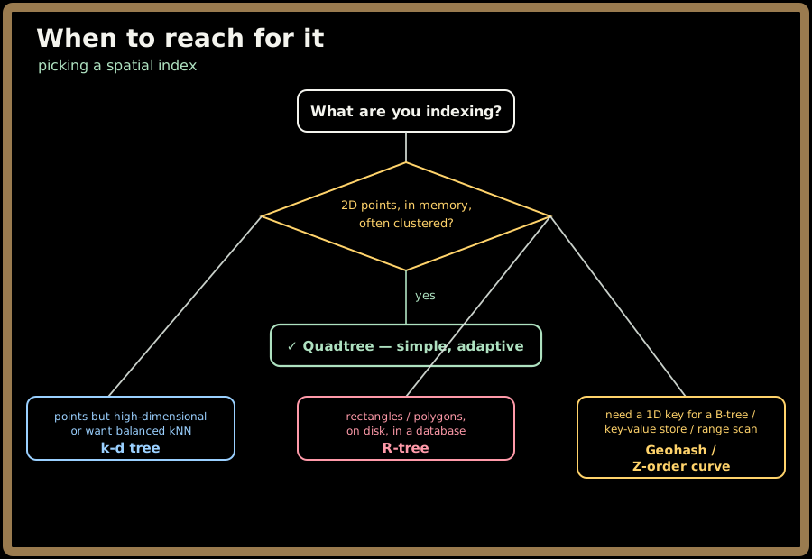
• k-d tree — splits on one dimension at a time (alternating x, y, x, y…) into two children, and picks the split at the median data point so the tree stays balanced. It scales to higher dimensions far better (a quadtree in d dimensions needs 2ᵈ children per node — 4 in 2D, but 8 for an octree, 16, 32… which explodes), and it's the classic choice for k-nearest-neighbour search. The catch: it's harder to keep balanced under lots of inserts and deletes. We compare these head-to-head in Part 3.
• R-tree — groups nearby objects into overlapping minimum bounding rectangles and is self-balancing (all leaves at the same depth), which makes it the standard on-disk, database spatial index (PostGIS, spatial databases). It handles extended objects (roads, polygons), not just points, and behaves well under updates. If your index lives in a database, it's probably an R-tree, not a quadtree.
• Geohash / Z-order curve — instead of a pointer tree, encode each (lat, lng) as a single string or integer by interleaving the bits of the two coordinates. That linearizes 2D space into a 1D key you can store in an ordinary B-tree, key-value store, or sharded database and range-scan — no custom in-memory tree required. This is the same recursive-quarter idea as a quadtree, just serialized; the dedicated Geohashing topic goes deep on it, and Part 3 shows why the two are two views of one concept.

⚠️ A quadtree is an in-memory, pointer-chasing structure. If you need it to survive a restart, shard across machines, or live inside a database, you usually don't ship a raw quadtree — you either use an R-tree (in the DB) or linearize with a geohash (in a KV store). Reaching for a hand-rolled quadtree as your system of record is a common junior mistake; it shines as an in-process index over data that lives somewhere durable.

---

Key takeaways

1. A quadtree recursively subdivides a 2D region into four quadrants (NW/NE/SW/SE), splitting a quadrant only when it exceeds its node capacity — so the tree is deep where data is dense and shallow where it's sparse.
2. It exists because 2D "nearness" isn't a 1D sort problem: a one-dimensional B-tree index can't answer "within 2 km" efficiently, and a linear scan is O(n). A quadtree prunes whole regions with one box-overlap test.
3. Know the three flavours: point (node is the data, like a 2D BST), region (uniform space split, used for image compression), and point-region (PR) — equal-quarter splits with points in capacity-bounded leaves, the one you mean for maps and find-nearby.
4. Query = prune: if a node's bounding box doesn't intersect your query rectangle, skip its entire subtree. That single check is the whole performance story.
5. Reach for a quadtree for in-memory, clustered 2D points; prefer a k-d tree for high-dimensional/kNN, an R-tree for on-disk/database and extended objects, and a geohash when you need a 1D key for a KV store — a connection we'll make precise later.

Next, Part 2 opens the hood: the exact node structure, the insert-and-split write path, how range queries and k-nearest-neighbour searches actually walk the tree, the complexity with real numbers, and the degenerate case that can quietly turn your O(log n) tree into an O(n) linked list.