Geohashing — Part 1: Foundations & Core Concepts

maang.io System Design Series

---

What is this?

Imagine a friend hides a pin somewhere on a world map and lets you find it with only yes/no questions — but there's a rule: every question must cut the current search area exactly in half. Your first question is "Is the pin in the eastern half of the world, or the western half?" East → you write down 1 and now only care about the eastern half. Next: "Is it in the northern half of what's left, or the southern half?" South → write 0. East-or-west again, north-or-south again, back and forth, each answer shrinking the box. After twenty questions your box is a tiny rectangle a few kilometres across; after forty it's smaller than your phone. The string of answers — 10110100… — is the location. And here's the magic: your friend's pin and your own location, if you're standing near each other, will produce almost the same string of answers, because you'd both answer the early questions identically.

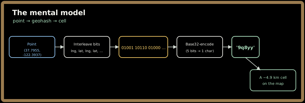
That guessing game is exactly what geohashing is. A geohash takes a (latitude, longitude) pair and encodes it as a short text string like 9q8yy by playing this halving game and writing the answers down — then packing every five answers into a single character so the string stays short. Two places that are near each other share a long prefix; two places far apart diverge early. That one property — shared prefix means physical proximity — is the entire reason geohashing exists, and it's what lets you answer "find everything near me" using nothing more than a plain string index in an ordinary database.

We'll keep coming back to this twenty-questions map game for the whole topic. It's the mental model that makes every later detail obvious.

The one-line idea: A geohash interleaves the bits of latitude and longitude and base32-encodes them into a short string, so that the longer the shared prefix between two geohashes, the closer the two points are on Earth — turning "who is near me?" into "who shares my string prefix?", a question any B-tree index already answers.

---

1. Why geohashing exists — what was painful before

Proximity search sounds trivial until you try to index it. Suppose you're building the "restaurants near me" feature. Every restaurant has a latitude and a longitude — two independent numbers. Your instinct is to put a B-tree index on each column (you met B-tree indexes in the 101 SQL chapter) and run:

SELECT * FROM places
WHERE lat BETWEEN 37.78 AND 37.81      -- a box around me
  AND lng BETWEEN -122.42 AND -122.39;

This works, but it's quietly awful at scale. A B-tree on lat can quickly find every place in that latitude band — but that band is a stripe wrapping the entire planet, from your city all the way around the globe. The lng index finds a second planet-wrapping stripe running the other way. The database has to pull one giant stripe and then filter it against the other, or intersect two enormous result sets. Neither index is selective on its own, because latitude alone and longitude alone each throw away half the information about where you are. You've indexed two 1-D numbers to answer an inherently 2-D question.

The deeper problem: a standard index sorts on one dimension, but "nearby" is a two-dimensional idea. You need a way to collapse two coordinates into one sortable key such that keys that are close in value are also close on the map. That's precisely the trick geohashing pulls off — it's a space-filling curve that threads through 2-D space in a 1-D order, so that a single ordinary index becomes a spatial index.

💡 The whole point of a geohash is to make an existing index type — the humble B-tree string index you already have in Postgres, MySQL, Cassandra, DynamoDB, or a Redis sorted set — behave like a spatial index, without adding a special spatial engine. Simplicity is the feature.

---

2. Core concepts & vocabulary — the mental model

Four ideas, and you're fluent.

Interleaving (the back-and-forth). In the guessing game we alternated: east/west (a longitude question), then north/south (a latitude question), then longitude again, then latitude again. Geohashing does the same — it interleaves longitude and latitude bits, taking turns bisecting each range. Longitude goes first. So the bit stream is lng, lat, lng, lat, ….

Base32 encoding (packing the answers). A raw stream of 30 or 40 bits is unwieldy, so geohash groups the bits into chunks of 5 and maps each chunk (a number 0–31) to one character using a special 32-character alphabet: 0123456789bcdefghjkmnpqrstuvwxyz. Notice it deliberately omits a, i, l, o — the letters most easily confused with digits or each other. Five bits per character is why every extra character adds five yes/no answers' worth of precision.

Precision = length (the box shrinks). Every character you add answers five more questions and shrinks the cell. The relationship is fixed and worth memorizing at a rough level:

Geohash length	Bits	Cell size (≈, at the equator)	Feels like
1	5	5,000 km × 5,000 km	a continent
2	10	1,250 km × 625 km	a large country
3	15	156 km × 156 km	a metro region
4	20	39 km × 20 km	a city
5	25	4.9 km × 4.9 km	a district
6	30	1.2 km × 0.61 km	a neighbourhood
7	35	153 m × 153 m	a city block
8	40	38 m × 19 m	a building
9	45	4.8 m × 4.8 m	a doorway

The one row to burn in: 6 characters ≈ a 1.2 km cell. That's the reference every engineer quotes.

The cell (a box, not a point). A geohash never names an exact point — it names the rectangular cell that the point fell into. 9q8yy isn't a coordinate; it's a ~4.9 km box, and every point inside that box shares the geohash 9q8yy. This is the same "you're not a point, you're a bucket" idea behind hashing generally — and it's what makes the prefix trick work: to zoom out to a coarser box, you just chop characters off the end. 9q8yy ⊂ 9q8y ⊂ 9q8 ⊂ 9q. Every cell nests perfectly inside its 5-bit-shorter parent, like Russian dolls.

---

3. How you actually use it — a concrete example

You store each place's geohash as an indexed string column, and you turn "near me" into a prefix match. Here's the whole idea in one table and one query:

CREATE TABLE places (
    id        bigint PRIMARY KEY,
    name      text,
    lat       double precision,
    lng       double precision,
    geohash   text            -- e.g. '9q8yyk8ytpxr', computed on write
);
CREATE INDEX idx_places_geohash ON places (geohash);   -- an ordinary B-tree

-- "Find places in roughly my ~5 km cell" — a prefix scan, which a B-tree
-- serves as a range scan (everything from '9q8yy' up to '9q8yz'):
SELECT id, name FROM places
WHERE geohash >= '9q8yy' AND geohash < '9q8yz';

Because a B-tree stores keys in sorted order, all rows sharing the prefix 9q8yy sit physically next to each other on disk — the query is one tight, sequential range scan instead of two planet-wrapping stripe intersections. That's the payoff: a spatial query served by a boring string index.

In application code the flow is: compute the querying point's geohash to your chosen precision, run the prefix scan, then filter the handful of candidates by true distance (the haversine formula) and sort. The geohash does the cheap coarse filtering (turn millions of rows into dozens); exact distance does the fine ranking on the survivors.

⚠️ There's one wrinkle you must know about even at the foundations level: a place 10 metres away from you, but just across a cell boundary, can have a completely different geohash with no shared prefix. So a single prefix scan can miss near neighbours that happen to sit in the adjacent box. The fix — querying your cell plus its 8 neighbours — is the "boundary problem," and it's important enough that we dedicate real time to it in Part 2. For now, just hold the caveat: one cell is a first cut, not the final answer.

---

4. When to reach for it — and when not

Geohashing is the right tool when you want proximity search inside an existing datastore without standing up specialized spatial infrastructure.

Reach for a geohash when:

• You need "find things near a point" or "things within N km," and N is roughly known.
• You want the spatial index to live as a plain string/number column in a DB you already run (Postgres, MySQL, Cassandra, DynamoDB) so it shards, replicates, and caches like any other data.
• You want proximity keys that are human-shareable and prefix-truncatable (a 4-char geohash is a coarse public location; more chars = more precise) — geo-URLs, tile keys, cache keys.
• You're building a fast pre-filter in front of exact-distance ranking.

Reach for something else when:

• You need adaptive resolution for wildly uneven density. A geohash grid uses the same box size everywhere, so a downtown cell holds a million points while an ocean cell holds zero. When you need the structure to subdivide only where it's crowded, a Quadtree (its own topic in this tier) is the better fit — it grows deep in dense areas and stays shallow in empty ones.
• You're on Redis and want it batteries-included. Redis ships geospatial commands (GEOADD, GEOSEARCH) that use geohashing under the hood — you get proximity search without hand-rolling any of this. We'll open that hood in Part 2 and Part 3.
• You need heavy-duty geo queries — polygon containment, routing, arbitrary shapes, "within this county boundary." That's a job for PostGIS, Elasticsearch geo queries, or Google's S2 / Uber's H3 libraries, not raw geohash prefixes.
• Equal-area or gap-free tiling matters (e.g. spatial aggregation). Geohash cells are rectangles that distort toward the poles; hexagonal systems like H3 handle that better.

At a glance:

If you need…	Reach for…
Proximity search in a plain DB index	Geohash
Density-adaptive subdivision, k-NN	Quadtree
Turnkey geo in a cache/store	Redis GEO (geohash inside)
Polygons, routing, rich GIS	PostGIS / Elasticsearch / S2 / H3

---

5. Key takeaways

1. A geohash is the twenty-questions map game written down: interleave the bits of longitude and latitude (lng first), base32-encode five bits per character, and you get a short string that names a rectangular cell, not a point.
2. Shared prefix = proximity. Two nearby places share a long prefix; that's what lets a plain B-tree string index answer spatial queries as a simple range/prefix scan — no special spatial engine required. That's the whole reason geohashing exists.
3. Length is precision: each character adds 5 bits and shrinks the cell. Memorize the anchor — 6 chars ≈ a 1.2 km cell — and interpolate from there.
4. Use it as a coarse pre-filter: prefix-scan to cut millions of rows to dozens, then rank the survivors by true (haversine) distance.
5. Know its edges: the boundary problem means one cell can miss a neighbour across the line (Part 2's headline), and a uniform grid can't adapt to density the way a Quadtree can. On Redis you often get all of this for free via Redis GEO.

Next, Part 2 cracks the encoding open: the exact bit-interleaving with a fully worked example, the Z-order space-filling curve that geohashes secretly trace, the boundary problem and the 9-cell neighbour query in detail, and how Redis turns all of this into a 52-bit score in a sorted set.